Week 4.1 - Genetic Algorithm

Aim:-Optimization of the stalagmite function and to find the global maxima of the function

Objective:-a)To write the code for optimization of the stalagmite function and explain the syntax of ga

b) To plot graphs for all three studies for F maximum and no of iterations

Theory:-The algorithm reflects the process of natural selection where the fittest individuals are selected for reproduction in order to produce offspring of the next generation.

Phases of genetic algorithm

1.Initial population

2.Fitness fuction

3.Selection

4.Crossover

5.Mutation

Syntax of ga

[x,fval,exitflag,output,population,scores]=ga(func,nvars,A,b,Aeq,Beq,lb,ub,nonlcon,lntcon,options)

x=optimum solution

exitflag= reason ga stopped

output=information about optimization process

population=final population

scores=final scores

f=ga(fun,nvars,Ab,[],[],lb,ub,nonlcon,lntcon,options)

fun=fitness function

nvars=number of variabels

A,b=linear inequality constraints

Aeq,beq=linear equality constraints

lb=lower bound(limit)

ub= upper bound(limit)

nonlcon=use for nonlinear constraints

lntcon=to get solution in integer

options=to set population size minimize with non default options

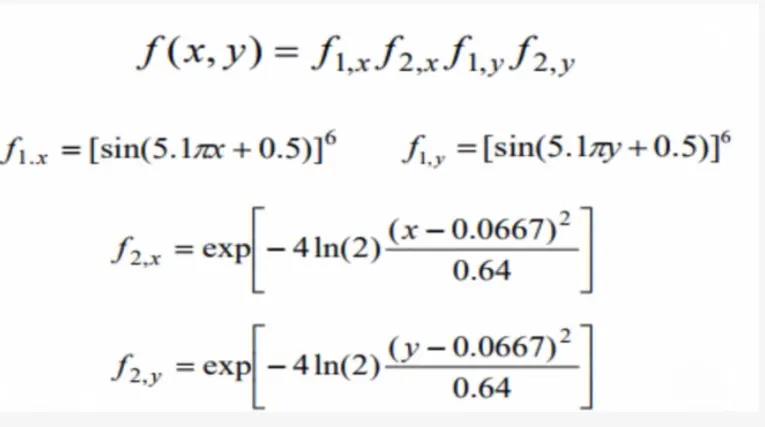
Fitness fuction used in our program

Procedure:-

1.The formula given above has been discreted and written as a function for the code

2.The code writtten for the function given is attached below

function

function [f]=stalagmite(input_vector)
x=input_vector(1);
y=input_vector(2);
f1_x=(sin(5.1*pi*x+0.5)).^6;
f1_y=(sin(5.1*pi*y+0.5)).^6;

t1=((x-0.0667).^2)/(0.64);
f2_x=exp(-4.*log(2)*t1);
t2=((y-0.0667).^2)/(0.64);
f2_y=exp(-4.*log(2)*t2);
f=-(f1_x.*f2_x.*f1_y.*f2_y);
end

3.code with given inputs to create surface plot of stalagmite

clear all
close all
clc
 x=linspace(0,0.6,150);
 y=linspace(0,0.6,150);
 
 [xx yy]=meshgrid(x,y);
 num_cases=50;
 
 for i=1:length(xx)
     for j=1:length(yy)
         input_vector(1)=xx(i,j);
         input_vector(2)=yy(i,j);
         f(i,j)=stalagmite(input_vector);
     end
 end
surfc(xx,yy,-f);
shading interp

4.code written for the statistical study in unbounded,bounded and increase in size of population conditions

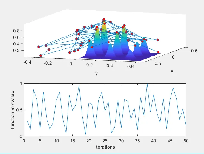
study1
%A program for statistical study in unboubed condition
clear all
close all
clc
% providing the search space for the function
 x=linspace(0,0.6,150);
 y=linspace(0,0.6,150);

 [xx, yy]=meshgrid(x,y); 
num_cases=50; %number of iterations for which the function will evaluate the fitness

%creating the surface plot of stalagmite function 
 for i=1:length(xx)
     for j=1:length(yy)
         input_vector(1)=xx(i,j);
         input_vector(2)=yy(i,j);
         f(i,j)=stalagmite(input_vector);
     end
 end
 %calculating the study time through tic and toc command 
tic
for i=1:num_cases
    [inputs,fval(i)]=ga(@stalagmite,2); %calculating the optimized vale of the function
    xopt(i)=inputs(1); %at each iterations
    yopt(i)=inputs(2);
end

study1_time=toc %displaying the time taken to evaluate

%plotting the graph
figure(1)
subplot(2,1,1)
hold on
surfc(xx,yy,-f);
shading interp
plot3(xopt,yopt,-fval,'marker','o','markersize',5,'markerfacecolor','r');
xlabel('x')
ylabel('y')
subplot(2,1,2)
plot(-fval);
xlabel('iterations')
ylabel('function minvalue')

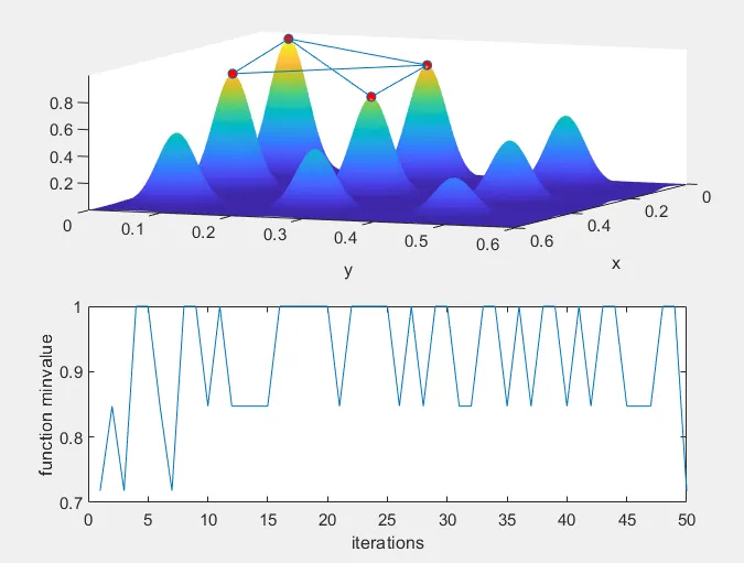
study2
%A program for statistical study in bounded condition
clear all
close all
clc
% providing the search space for the function
 x=linspace(0,0.6,150);
 y=linspace(0,0.6,150);

 [xx, yy]=meshgrid(x,y);
num_cases=50;  %number of iterations for which the function will evaluate the fitness

%creating the surface plot of stalagmite function 
 for i=1:length(xx)
     for j=1:length(yy)
         input_vector(1)=xx(i,j);
         input_vector(2)=yy(i,j);
         f(i,j)=stalagmite(input_vector);
     end
 end
  %calculating the study time through tic and toc command 
tic
for j=1:num_cases
    [inputs,fval(j)]=ga(@stalagmite,2,[],[],[],[],[0;0],[1;1]);%calculating the optimized vale of the function
    xopt(j)=inputs(1);
    yopt(j)=inputs(2);
end

study2_time=toc %displaying the time taken to evaluate

%plotting the graph
figure(1)
subplot(2,1,1)
hold on
surfc(xx,yy,-f);
shading interp
plot3(xopt,yopt,-fval,'marker','o','markersize',5,'markerfacecolor','r');
xlabel('x')
ylabel('y')
subplot(2,1,2)
plot(-fval);
xlabel('iterations')
ylabel('function minvalue')

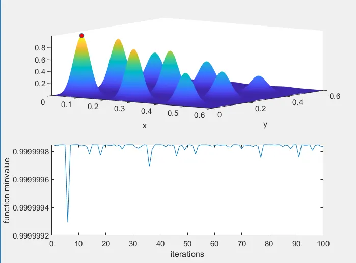
study3
% A program for statistical study with increase in size of population
clear all
close all
clc
% providing the search space for the function
 x=linspace(0,0.6,150);
 y=linspace(0,0.6,150);

 [xx, yy]=meshgrid(x,y);
num_cases=100; %number of iterations for which the function will evaluate the fitness

%creating the surface plot of stalagmite function 
 for i=1:length(xx)
     for j=1:length(yy)
         input_vector(1)=xx(i,j);
         input_vector(2)=yy(i,j);
         f(i,j)=stalagmite(input_vector);
     end
 end
 options=optimoptions('ga','populationsize',300)
  %calculating the study time through tic and toc command 
tic
for k=1:num_cases
    [inputs,fopt(k)]=ga(@stalagmite,2,[],[],[],[],[0;0],[1;1],[],[],options);%calculating the optimized vale of the function
    xopt(k)=inputs(1);
    yopt(k)=inputs(2);
end

study3_time=toc %displaying the time taken to evaluate

%plotting the graph
figure(3)
subplot(2,1,1)
hold on
surfc(xx,yy,-f);
shading interp
plot3(xopt,yopt,-fopt,'marker','o','markersize',5,'markerfacecolor','r');
xlabel('x')
ylabel('y')
subplot(2,1,2)
plot(-fopt);
xlabel('iterations')
ylabel('function minvalue')

5.Linspace command is used to define x and y with 150 elements between 0 and 0.6 including the bounds

6.Then num_cases is set which will be used as counter for iterations to 50(bounded & unbounded condition) 100(increase in size of population condition)

7.2D gird is made using meshgrid command is created from x and y input to be outputted to xx and yy

8.To create the surface plot surfc command in used

9.Tic and toc command is used to calculate the time taken for study of each individual conditions in the code

10.Nested loop is used in the code

11.By providing the upper and lower limit in the ga ,the serach space is reduced with upper and lower boundary

12.The variation in optimum value is redudced by providing the boundary conditions

13.Optimoptions command is used to increase the size of the population

14.Negative sign(-)is used in the fval or fopt to find the maximum value

15.subplot command is used to plot two graphs at same window

Results

The time taken for evaluation in each condition is given below:-

study_time1=4.8131

study_time2=6.836

study_time3=48.2363

The stalagmite plot as been obtained for all three conditions with maxima value

Plots

study1

study 2

study3

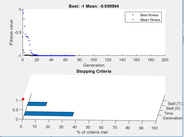
stopping criteria

Conclusion

1.This genetic algorithm tries to maximize the fitness function to provide a population consisting of the fittest individual by optimizing the function.

2.The fitness has been calculated and the best result has been displayed even with the reduction in size of the population