Week 3 - Solving second order ODEs

Aim:- To write a program in matlab to simulate the pendulum motion

Objective:-a)To solve the ode which represents the equation of motion of a simple pendulum with damping

b)To animate the motion of the pendulum

Theory:- Pendulum is an ideal model in which the material point of mass m is suspended on a weightless and inextensible string of length L. In this system, there are periodic oscillations, which can be regarded as a rotation of the pendulum about the axis

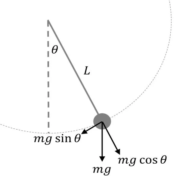
The second order differential equation used here is:-

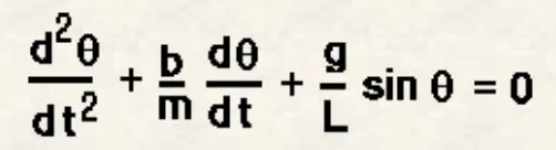
In the above equation,

g=gravity in m/s^2

m=mass of the ball in kg

L=length of the pendulum in m

b= damping coefficient

%Inputs

damping coefficient (b)=0.05

length of the pendulum (l)=1m

mass of the ball (m)=1kg

gravity (g)=9.81m/s^2

angular displacement = 0

angular velocity= 3 rad/sec at t=0

for a time period=0-20 sec

Procedure:-

1.solve the given second order ode by breaking it into the series of first order ode

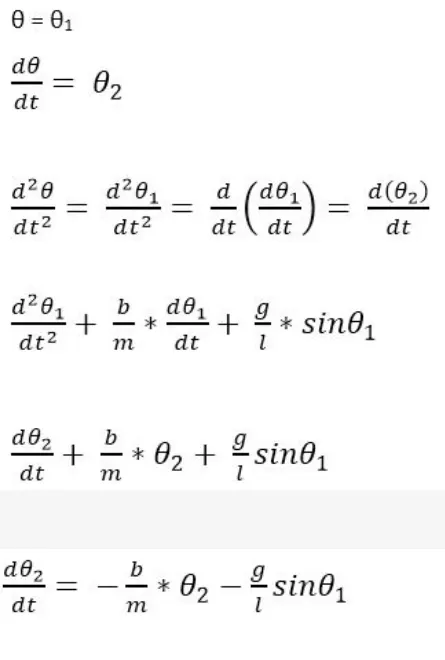
2.Creating the matrix form from the obtained equation

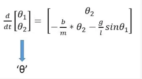
3.write the matlab program from the given inputs and obtained equation

code:-

% a program to simulate the pendulum motion 

clear all 
close all 
clc

%inputs

%damping co_efficient
b=0.05; 
%gravity
g=9.81;
%length of the pendulum
l=1;
%mass
m=1;

% initial condition 
theta_0=[0;3]; %angular displacement=0 %angular velocity=3

% time points
t_span=linspace(0,20,500);%time integrate

%solve ode
[t,results]=ode45(@(t,theta)ode_pendulum(t,theta,b,g,l,m),t_span,theta_0);

%plotting

figure(1)
%time vs displacement
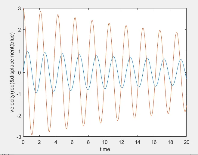
plot(t,results(:,1))
hold on
%time vs angular velocity
plot(t,results(:,2))
xlabel('time')
ylabel('velocity(red)&displacement(blue)')

%animation
ct=1;
for i=1:length(results(:,1))
x0=0
y0=0
x1=1*sin(results(i,1));
y1=-1*cos(results(i,1));
figure(2) 
%creating a beam
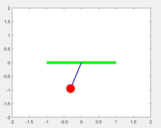
plot([-1 1],[0 0],'linewidth',6,'color','g');
%fixed axis
axis([-2 2 -2 2]);
%creating the line from initial value to final value
line([x0 x1],[y0 y1],'linewidth',2,'color','b');
hold on;
%creating the sphere at the end of the string
plot(x1,y1,'marker','o','markerSize',20,'markerFacecolor','r');
pause(0.1)
%for anime
z(ct)=getframe(gcf);
ct=ct+1;
hold off;
end

%animation converted
movie(z)
videofile=VideoWriter('pendulum.avi','uncompressed AVI');
open(videofile)
writeVideo(videofile,z)
close(videofile)

The function of ode_pendulum:-

function[dtheta_dt]=ode_pendulum(t,theta,b,g,l,m)
theta1=theta(1)
theta2=theta(2)
dtheta1_dt=theta2;
dtheta2_dt=-(b/m)*theta2-(g/l)*sin(theta1);
dtheta_dt=[dtheta1_dt;dtheta2_dt];
end

4.Required initial conditions and inputs have been added to the code

5.Time span command has been used ,500 values as been taken in the time period of 0-20 secs

6.ode45 command is used to add the ode function in the program with the required inputs

7.plotting as been done with respect to time vs angular velocity and time vs angular displacement

8.For loop command is used to mark the mass at various points and time, has been plotted in the graph

9.Marker command is used to create the sphere

10.Using movie command the animation of pendulum as been created and saved as an uncompressed avi file

Outputs:-

1.plot

Conclusion:-1.The simulation of the pendulum as been obtained with the time interval of 0-20 secs

2. The animation of the motion of pendulum is created,it has been saved as a avi file and attached in the google drive link below

Animated link

https://drive.google.com/file/d/12wX6g-Kz4U0XyeJsP4P7_ldEuyHiEb6U/view?usp=sharing