Week 4.1 - Genetic Algorithm

GENETIC ALGORITHM

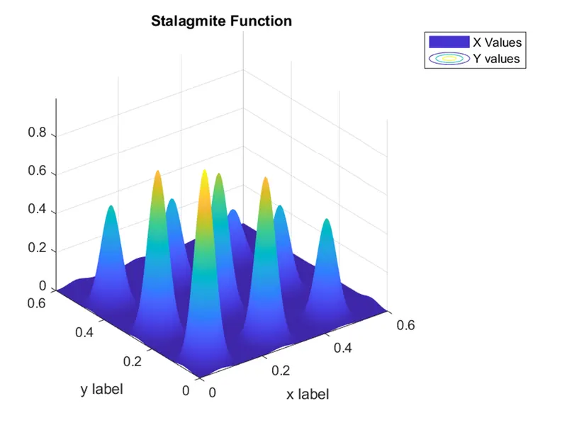
AIM: To write a MATLAB program to optimize the stalagmite function and find the global maxima of the function.

OBJECTIVE: to optimize the Stalagmite function and find the global maxima of the function by clearly explaining the concept of genetic algorithm and plotting the graph for the three studies i.e. unbounded inputs, bounded inputs, and bounded inputs with modified population size.

THEORY:

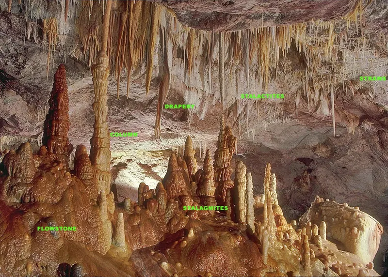
Stalagmites: A Stalagmite is a type of rock formation that rises from the floor of a cave due to the accumulation of material deposited on the floor from ceiling drippings. Stalagmites are typically composed of calcium carbonate but may consist of lava, mud, peat, pitch, sand, sinter, and amberat (crystallized urine of packrats).

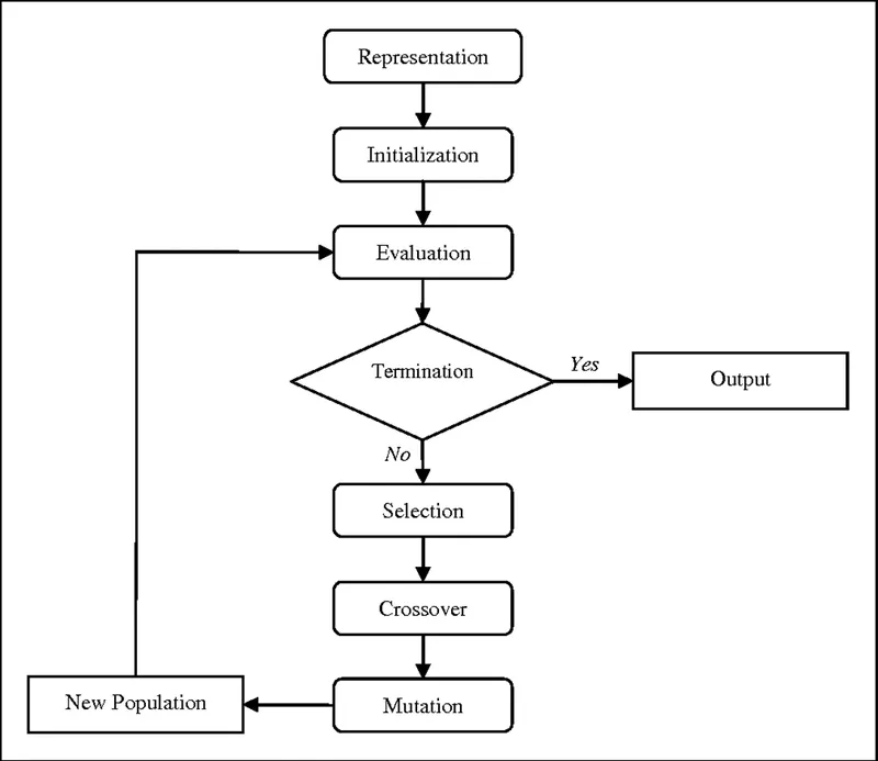
Genetic Algorithm: In computer science and operations research, a genetic algorithm (GA) is a metaheuristic inspired by the process of natural selection that belongs to the larger class of evolutionary algorithms (EA). Genetic algorithms are commonly used to generate high-quality solutions to optimization and search problems by relying on biologically inspired operators such as mutation, crossover, and selection.

It is inspired by Charles Darwin's theory of natural evolution. This algorithm reflects the process of natural selection where the fittest individuals are selected for reproduction to produce offspring of the next generation.

Charles Darwin's Theory of Natural Evolution: The theory of evolution by natural selection, first formulated in Darwin's book "On the Origin of Species" in 1859, is the process by which organisms change over time as a result of changes in heritable physical or behavioral traits. Changes that allow an organism to better adapt to its environment will help it survive and have more offspring.

Evolution by natural selection is one of the best-substantiated theories in the history of science, supported by evidence from a wide variety of scientific disciplines, including paleontology, geology, genetics, and developmental biology.

WORKING PRINCIPLE: Genetic algorithms (GAs) are stochastic search methods based on the principles of natural genetic systems. They perform a search in providing an optimal solution for the evaluation (fitness) function of an optimization problem. GAs deal simultaneously with multiple solutions and use only the fitness function values. While solving an optimization problem using GAs, each solution is coded as a string (called "chromosome") of finite length over a finite alphabet A. Each string or chromosome is considered an individual. A collection of M (M is finite) such individuals is called a population.

The genetic algorithm starts with a randomly generated population of size M. During the process of iteration, a new population of the same size is generated from the current population using three basic operations on the individuals of the population.

Five phases are considered in a genetic algorithm.

1. Initial Population
2. Fitness function
3. Selection
4. Crossover
5. Mutation

Initial Population: The process begins with a set of individuals which is called a Population. Each individual is a solution to the problem you want to solve. An individual is characterized by a set of parameters (variables) known as Genes. Genes are joined into a string to form a Chromosome (solution). In a genetic algorithm, the set of genes of an individual is represented using a string, in terms of an alphabet. Usually, binary values are used (strings of 1s and 0s). We say that we encode the genes in a chromosome.

Fitness function: The fitness function determines how to fit an individual is (the ability of an individual to compete with other individuals). It gives a fitness score to each individual. The probability that an individual will be selected for reproduction is based on its fitness score.

Selection: The idea of the selection phase is to select the fittest individuals and let them pass their genes to the next generation. Two pairs of individuals (parents) are selected based on their fitness scores. Individuals with high fitness have more chances to be selected for reproduction.

Crossover: Crossover is the most significant phase in a genetic algorithm. For each pair of parents to be mated, a crossover point is chosen at random from within the genes.

Mutation: In certain new offspring formed, some of their genes can be subjected to a mutation with a low random probability. This implies that some of the bits in the bit string can be flipped.

Equations Used:

The Function is for the Genetic Algorithm of the global minima but in order to attain the maxima value the ‘-’ is placed before the equation.

f(x,y)=f1.x×f2.x×f1.y×f2.y

where,

f1.x=[sin(5.1πx+0.5)]6

f1.y=[sin(5.1πy+0.5)]6

f2.x=exp[−4ln(2)×(x−0.0667)20.64]

f2.y=exp[−4ln(2)×(y−0.0667)20.64]

The global maxima are as follows,

f(x,y)=−(f1.x×f2.x×f1.y×f2.y)

Process of Solving:

The Order in which the code is written is as below

1. Write Stalagmite Function.
2. Evaluating the stalagmite function.
3. Writing the code for Unbounded Inputs.
4. Writing the code for the Bounded Inputs.
5. Writing the code for the Bounded Inputs with modified population size.

PROCEDURE:

1. Writing the Stalagmite Function – The Stalagmite function is a core part of the code. The function follows the formula stated in the Equation used. The ‘Function’ input is used to write a function code.

function [f] = stalagmite(input_vector)

x= input_vector(1);
y= input_vector(2);

f1 = (sin(5.1*pi*x + 0.5)).^6;
f2 = exp(-4*log(2)*((x-0.0667).^2)./0.64);
f3 = (sin(5.1*pi*y + 0.5)).^6;
f4 = exp(-4*log(2)*((y-0.0667).^2)./0.64);

f = -(f1*f2*f3*f4);

end

2. Evaluating the Stalagmite function – The code is written to check if the function is returning an output. The function creates a 3D plot showing the Algorithm.

%Initial input Values 
lower_bound= input('Enter the Lower Bound Value: ');
upper_bound= input('Enter the Upper Bound Value: ');

% Input Variables with proper line spaces
x= linspace(lower_bound,upper_bound,150);
y= linspace(lower_bound,upper_bound,150);

% 3D Matrix creation
[xx, yy] = meshgrid(x,y);


count = 50;     % Giving the Count/ Number of Iterations for the optimal generation
tic             % Tic Starts the Clock time for the function
for i = 1:length(xx)
    for j=1:length(yy)
        input_vector(1)= xx(i,j);
        input_vector(2)= yy(i,j);
        f(i,j)=stalagmite(input_vector);
    end
end

study_time = toc;   % Toc stops the timer and shows the end time 
figure(1)
surfc(xx,yy,-f)
shading interp
xlabel('x label')
ylabel('y label')
legend('X Values','Y values')
title('Stalagmite Function')
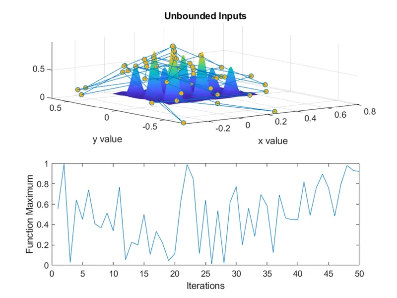
saveas(1, 'Stalagmite.png')

3. Writing the code for Unbounded inputs – For the Unbounded Stalagmites, the code starts with a ‘for’ loop having the inputs and optimal function with calling the function. Ga is explained clearly in the ‘Terms used’. The plot is generated with unbounded stalagmite

%Study 1 Unbounded/random sampling Inputs
tic

for i= 1:count
    [inputs,fopt(i)]= ga(@stalagmite,2);
    xopt(i)= inputs(1);
    yopt(i)= inputs(2);
end

studytime_1 =toc;

figure(2)
subplot(2,1,1)
surfc(x,y,-f)
shading interp
title('Unbounded Inputs')
xlabel('x value')
ylabel('y value')

hold on 
plot3(xopt,yopt,-fopt,'marker','o', 'markersize',5,'markerfacecolor','#EDB120');
subplot(2,1,2)
plot(-fopt)
xlabel('Iterations')
ylabel('Function Maximum')
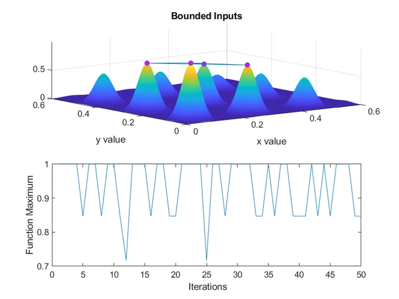
saveas(2,'Unbound Inputs.png')

4. Writing the code for Bounded inputs – The code is written for the genetic algorithm function built-in inside the MATLAB. An empty array is created with starting and ending points of the x and y values. The plot is created with the inputs in the proper order.

%Study 2 - Statistical Behaviour With upper and lower Bound sampling 
%(Bounded Inputs)

tic
for i = 1:count
    [inputs, fopt(i)]= ga(@stalagmite, 2, [],[],[],[], [lower_bound;lower_bound],[upper_bound;upper_bound]);
    xopt(i)= inputs(1);
    yopt(i)= inputs(2);
end
studytime_2 = toc;

figure(3)
subplot(2,1,1) 
surfc(x,y,-f)
shading interp
title('Bounded Inputs')
xlabel('x value')
ylabel('y value')

hold on

plot3(xopt,yopt,-fopt, 'marker','o', 'markersize', 5, 'markerfacecolor', 'm')
subplot(2,1,2)
plot(-fopt)
xlabel(' Iterations' )
ylabel('Function Maximum')
saveas(3, 'Bounded Input.png')

5. Writing the code for the Bounded Inputs with modified population size – The code begins with writing ‘optimoptions’. The details are given in the ‘Terms used’. The plot is then created as the previous method. The Global Maxima is calculated.

%Study 3 - code for Upper and Lower bound sampling and increase the
%population size
options = optimoptions(@ga);
options = optimoptions(options,'populationsize',170);

tic;
for i=1:count
    [inputs,fopt(i)]= ga(@stalagmite,2,[],[],[],[],[lower_bound;lower_bound],[upper_bound;upper_bound],[],[],options);
    xopt(i)= inputs(1);
    yopt(i)= inputs(2);
end

studytime_3 = toc;
figure(4)
subplot(2,1,1)
surfc(x,y,-f)
shading interp
title('Bounded Inputs with modified population size')
xlabel('x value')
ylabel('y value')

hold on 

plot3(xopt,yopt,-fopt, 'marker','o','markersize',5,'markerfacecolor','c')
subplot(2,1,2)
plot(-fopt)
xlabel('Iterations')
ylabel('Function Maxima')
saveas(4, 'Bounded Inputs with modified population size.png')

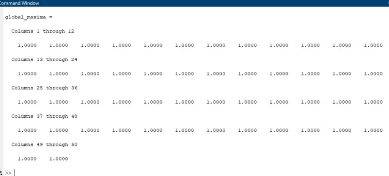
global_maxima = -fopt       % Finding the Global Maxima

CODE

• FOR FUNCTION:

function [f] = stalagmite(input_vector)

x= input_vector(1);
y= input_vector(2);

f1 = (sin(5.1*pi*x + 0.5)).^6;
f2 = exp(-4*log(2)*((x-0.0667).^2)./0.64);
f3 = (sin(5.1*pi*y + 0.5)).^6;
f4 = exp(-4*log(2)*((y-0.0667).^2)./0.64);

f = -(f1*f2*f3*f4);

end

• FOR MAIN FUNCTION:

clear
close
clc

%Initial input Values 
lower_bound= input('Enter the Lower Bound Value: ');
upper_bound= input('Enter the Upper Bound Value: ');

% Input Variables with proper line spaces
x= linspace(lower_bound,upper_bound,150);
y= linspace(lower_bound,upper_bound,150);

% 3D Matrix creation
[xx, yy] = meshgrid(x,y);


count = 50;     % Giving the Count/ Number of Iterations for the optimal generation
tic             % Tic Starts the Clock time for the function
for i = 1:length(xx)
    for j=1:length(yy)
        input_vector(1)= xx(i,j);
        input_vector(2)= yy(i,j);
        f(i,j)=stalagmite(input_vector);
    end
end

study_time = toc;   % Toc stops the timer and shows the end time 
figure(1)
surfc(xx,yy,-f)
shading interp
xlabel('x label')
ylabel('y label')
legend('X Values','Y values')
title('Stalagmite Function')
saveas(1, 'Stalagmite.png')
% [x, fval]= ga(@stalagmite,2)


%Study 1 Unbounded/random sampling Inputs
tic

for i= 1:count
    [inputs,fopt(i)]= ga(@stalagmite,2);
    xopt(i)= inputs(1);
    yopt(i)= inputs(2);
end

studytime_1 =toc;

figure(2)
subplot(2,1,1)
surfc(x,y,-f)
shading interp
title('Unbounded Inputs')
xlabel('x value')
ylabel('y value')

hold on 
plot3(xopt,yopt,-fopt,'marker','o', 'markersize',5,'markerfacecolor','#EDB120');
subplot(2,1,2)
plot(-fopt)
xlabel('Iterations')
ylabel('Function Maximum')
saveas(2,'Unbound Inputs.png')

%Study 2 - Statistical Behaviour With upper and lower Bound sampling 
%(Bounded Inputs)

tic
for i = 1:count
    [inputs, fopt(i)]= ga(@stalagmite, 2, [],[],[],[], [lower_bound;lower_bound],[upper_bound;upper_bound]);
    xopt(i)= inputs(1);
    yopt(i)= inputs(2);
end
studytime_2 = toc;

figure(3)
subplot(2,1,1) 
surfc(x,y,-f)
shading interp
title('Bounded Inputs')
xlabel('x value')
ylabel('y value')

hold on

plot3(xopt,yopt,-fopt, 'marker','o', 'markersize', 5, 'markerfacecolor', 'm')
subplot(2,1,2)
plot(-fopt)
xlabel(' Iterations' )
ylabel('Function Maximum')
saveas(3, 'Bounded Input.png')


%Study 3 - code for Upper and Lower bound sampling and increase the
%population size
options = optimoptions(@ga);
options = optimoptions(options,'populationsize',170);

tic;
for i=1:count
    [inputs,fopt(i)]= ga(@stalagmite,2,[],[],[],[],[lower_bound;lower_bound],[upper_bound;upper_bound],[],[],options);
    xopt(i)= inputs(1);
    yopt(i)= inputs(2);
end

studytime_3 = toc;
figure(4)
subplot(2,1,1)
surfc(x,y,-f)
shading interp
title('Bounded Inputs with modified population size')
xlabel('x value')
ylabel('y value')

hold on 

plot3(xopt,yopt,-fopt, 'marker','o','markersize',5,'markerfacecolor','c')
subplot(2,1,2)
plot(-fopt)
xlabel('Iterations')
ylabel('Function Maxima')
saveas(4, 'Bounded Inputs with modified population size.png')

global_maxima = -fopt       % Finding the Global Maxima

TERMS USED:

1. Ga: Ga function is used to find the minimum of the function using a genetic algorithm.

Syntax –

1. For Random Inputs: x = ga(fun,nvars)finds a local unconstrained minimum, x, to the objective function, f;un. nvars is the dimension (number of design variables) of
2. For Bounded Inputs: x = ga(fun,nvars,A,b,Aeq,beq,lb,ub)defines a set of lower and upper bounds on the design variables, x, so that a solution is found in the range lb ≤ x ≤ ub. (Set Aeq= [] and beq= [] if no linear equalities exist.)

• For Population size: x = ga(fun,nvars,A,b,[],[],lb,ub,nonlcon,IntCon,options)requires that the variables listed in IntCon take integer values.

where,

Fun – function,

Nvars – Number of Variables

A – Linear inequality constraints

B – Linear inequality constraints

Aeq - linear equality constraints

beq – linear equality constraints

lb – lower Bounds

ub – Upper Bounds

nonlcon – Non- Linear Constraints

IntCon – Integer Constraints

2. Surfc: surfc function contours the plot under the surface plot. surfc(X, Y, Z)creates a three-dimensional surface plot with a contour plot underneath. A surface plot is a three-dimensional surface that has solid edge colors and solid face colors. The function plots the values in matrix Z as heights above a grid in the x-y plane defined by X and Y. The color of the surface varies according to the heights specified by Z.
3. Shading: The shading function controls the color shading of surface and patch graphics objects.

Shading flat each mesh line segment and face has a constant color determined by the color value at the endpoint of the segment or the corner of the face that has the smallest index or indices.

shading faceted flat shading with superimposed black mesh lines. This is the default shading mode.

shading interp varies the color in each line segment and face by interpolating the colormap index or true color value across the line or face

shading(axes_handle,...) applies the shading type to the objects in the axes specified by axes_handle, instead of the current axes. Use single quotes when using a function form. For example: shading(gca,'interp')

4. Plot3: plot3(X, Y, Z) plots coordinates in 3-D space.

To plot a set of coordinates connected by line segments, specify X, Y, and Z as vectors of the same length. To plot multiple sets of coordinates on the same set of axes, specify at least one of X, Y, or Z as a matrix and the others as vectors.

5. Optimoptions: options = optimoptions(SolverName) returns a set of default options for the SolverName solve

options = optimoptions(oldoptions,Name,Value) returns a copy of oldoptions with the named parameters altered with the specified values.

6. Tic-Toc: tic works with the toc function to measure elapsed time. The 'tic' function records the current time, and the toc function uses the recorded value to calculate the elapsed time.

toc reads the elapsed time since the stopwatch timer started by the call to the tic function. MATLAB reads the internal time at the execution of the toc function and displays the elapsed time since the most recent call to the tic function without an output. The elapsed time is expressed in seconds.

RESULTS:

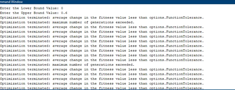
The results show the generation of the stalagmites. The start and end boundaries are taken as inputs

The random sampling output is shown below:

The Bounded samples output is shown below:

The Bounded samples output with the given population size is shown below:

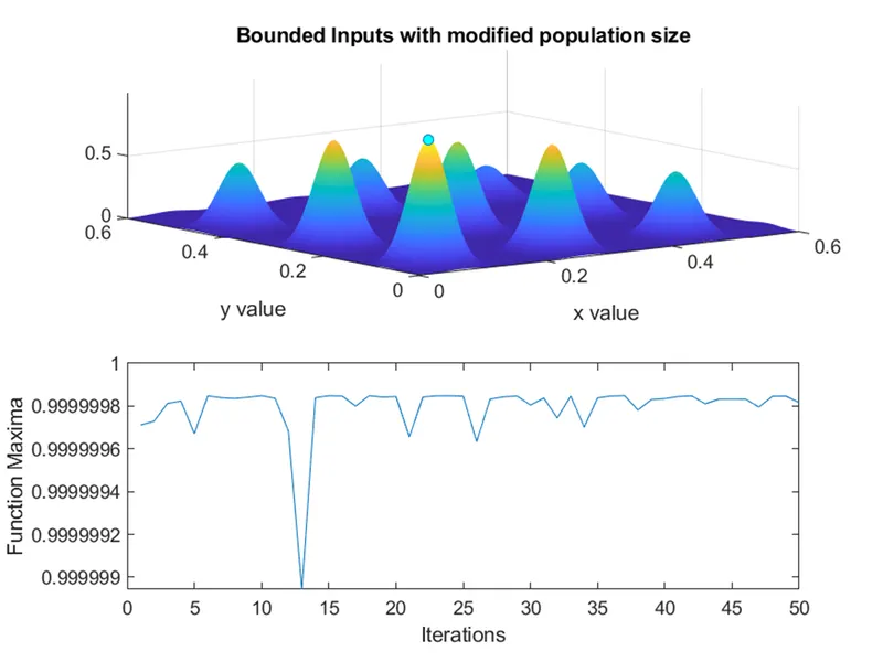
The above results show that the bounded samples with population size have an accurate solution. This is because the code shows the random samples which can start and end at random points.

To overcome the issue, the bounded samples method is used giving the lower and upper limits. (Therefore, it will take the values which are greater than the upper bound or less than the lower bound.)

This loop gives an output with different local maxima with bounded inputs. To conquer this problem, we need to increase the population size as it increases the probability to converge to a global maximum.

The Global maximum of a function can be found by inverting the function. Find the minimum value of the inverted function, the negative of the minimum value will give the global maximum of the function.

ERRORS:

The Errors were made which were simple syntax errors that are rectified right away with the help of the instructions in the command window.

References:

Stalagmite: Stalagmite – Wikipedia

Genetic Algorithm: Genetic Algorithm – Wikipedia

Introduction to Genetic Algorithm: The content for the genetic algorithm syntax, surfc, and other expressions were searched from the Help desk in MATLAB.