Challenge

Week 4.1 - Genetic Algorithm

JJitendra Sinha20 Jul 2022

Stalagmite

A stalagmite is a type of rock that rises from the floor of a cave due to the accumulation of materials decomposed on the floor from ceiling drippings.

That is why we are using the stalagmite as the name for the program due to its shape.

Introduction to Optimization

Optimization is the process of making something better. and it is decision making process.
In any process, we have a set of inputs and a set of outputs .
optimization help to find the best value for length breadth and width of the any structure and structure factor of safety, material consumed and stress induced are within the limit.

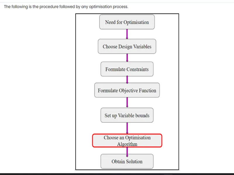
Techniques avilable to perform optimisation:-

Deterministic method:- e.g.-stress anaysis
Stochastic method:-it is predictive method and having probabilistic approch.

Genetic Algoritham(ga)

Genetic Algorithm (GA) is a search-based optimization technique.
it is based on the principles of Genetics and Natural Selection.
They help solve optimisation and search problems.
Genetec algoritham imitates natural biological process such as inheritance , mutation , selection and crossover.
The concept of algoritham is a search technique often used compute science to find complex non-obvious solution to algorithamic optimisation and search problems.

MATHEMATICAL EQUATION:

To find global maxima

f=(f1⋅f2⋅f3⋅f4)f=(f1⋅f2⋅f3⋅f4)

To find global minima

f=−(f1⋅f2⋅f3⋅f4)f=-(f1⋅f2⋅f3⋅f4)

where

f1=[sin(5.1πx+0.5)]6f1=[sin(5.1πx+0.5)]6

f2=[sin(5.1πy+0.5)]6f2=[sin(5.1πy+0.5)]6

f3=exp[−4log(2)(x−0.0667)20.64]f3=exp[-4log(2)(x-0.0667)20.64]

f4=exp[−4log(2)((y−0.0667)20.64)]f4=exp[-4log(2)((y-0.0667)20.64)]

here x and y are two variables

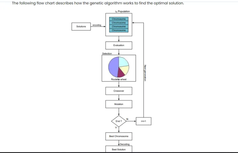
The genetic algorithm uses three main types of rules at each step to create the next generation from the current population:
- Selection rules select the individuals, called parents, that contribute to the population at the next generation.
- Crossover rules combine two parents to form children for the next generation.
- Mutation rules apply random changes to individual parents to form children.

‘’Syntax for GA’’

fitness fcn	Fitness functions
nvars	Number of design variables
Aineq	A matrix for linear inequality constraints
Bineq	b vector for linear inequality constraints
Aeq	Aeq matrix for linear equality constraints
Beq	beq vector for linear equality constraints
lb	Lower bound on x
ub	Upper bound on x
nonlcon	Nonlinear constraint function
rngstate	Optional field to reset the state of the random number generator
solver	'ga'
options	Options created using optimoptions or exported from the Optimization app

x= ga(fun,nvars) finds a local unconstrained minimum, x, to the objective function, fun. nvars is the dimension (number of design variables) of fun.
x= ga(fun,nvars,A,b) finds a local minimum x to fun, subject to the linear inequalities A*x ≤ b. ga evaluates the matrix product A*x as if x is transposed (A*x').
x= ga(fun,nvars,A,b,Aeq,beq) finds a local minimum x to fun, subject to the linear equalities Aeq*x = beq and A*x ≤ b. (Set A=[] and b=[] if no linear inequalities exist.) ga evaluates the matrix product Aeq*x as if x is transposed (Aeq*x').
x= ga(fun,nvars,A,b,Aeq,beq,lb,ub) defines a set of lower and upper bounds on the design variables, x, so that a solution is found in the range lb ≤ x ≤ ub. (Set Aeq=[] and beq=[] if no linear equalities exist.)
x= ga(fun,nvars,A,b,Aeq,beq,lb,ub,nonlcon) subjects the minimization to the constraints defined in nonlcon. The function nonlcon accepts x and returns vectors C and Ceq, representing the nonlinear inequalities and equalities respectively. ga minimizes the fun such that C(x) ≤ 0 and Ceq(x) = 0. (Set lb=[] and ub=[] if no bounds exist.)
x= ga(fun,nvars,A,b,Aeq,beq,lb,ub,nonlcon,options) minimizes with the default optimization parameters replaced by values in options. (Set nonlcon=[] if no nonlinear constraints exist.) Create options using optimoptions.
x= ga(fun,nvars,A,b,[],[],lb,ub,nonlcon,IntCon) or x = ga(fun,nvars,A,b,[],[],lb,ub,nonlcon,IntCon,options) requires that the variables listed in IntCon take integer values.
x= ga(problem) finds the minimum for problem, where problem is a structure.
[x,fval] = ga(___), for any previous input arguments, also returns fval, the value of the fitness function at x.
[x,fval,exitflag,output] = ga(___) also returns exitflag, an integer identifying the reason the algorithm terminated, and output, a structure that contains output from each generation and other information about the performance of the algorithm.
[x,fval,exitflag,output,population,scores] = ga(___) also returns a matrix population, whose rows are the final population, and a vector scores, the scores of the final population.

Errors :- error in the spelling .

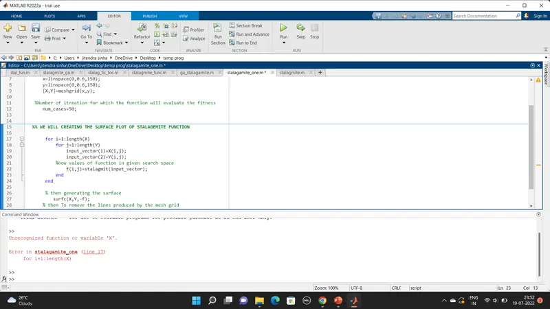
errors in the 17th line , it is not error , i resolve the error to select the all program and run then program was not showing errors .

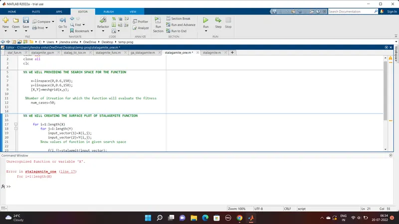
Errors resolve :-

at the function spelling "e" is missing so that error in program now we can correct the spelling ,and run the program .

process of the program :-

in the below first we make function formula , and attech the main cod as same file name .

% we start clear all, close all , clc .

%WE WILL PROVIDING THE SEARCH SPACE FOR THE FUNCTION

%Number of itreation for which the function will evaluate the fitness

%% WE WILL CREATING THE SURFACE PLOT OF STALAGEMITE FUNCTION

in the urface plot we used for loop and for loop or function formula

%now values of function in given search space

% then generating the surface

% then To remove the lines produced by the mesh grid

%tital of graph

first code

function [f] = stalagmite(input_vector)
          
            x = input_vector(1);
            y = input_vector(2);
 
            f1_x = (sin(5.1*pi*x + 0.5)).^6;
            f1_y = (sin(5.1*pi*y + 0.5)).^6;
 
            t1 = ((x-0.0667).^2)/(0.64);
            f2_x = exp(-4.*log(2)*t1);
 
            t2 = ((y-0.0667).^2)/(0.64);
            f2_y = exp(-4.*log(2)*t2);
 
            f = -(f1_x.*f2_x.*f1_y.*f2_y);
           
end

-:now we can use the function :-

clear all
close all
clc

%% WE WILL PROVIDING THE SEARCH SPACE FOR THE FUNCTION

    x=linspace(0,0.6,140);
    y=linspace(0,0.6,140);
    [X,Y]=meshgrid(x,y);
    
 %Number of itreation for which the function will evaluate the fitness
    num_cases=40;      


%% WE WILL CREATING THE SURFACE PLOT OF STALAGEMITE FUNCTION

     for i=1:length(X)
         for j=1:length(Y)
             input_vector(1)=X(i,j);
             input_vector(2)=Y(i,j);
         %now values of function in given search space
             f(i,j)=stalagmit(input_vector);  
         end
     end
 
     % then generating the surface
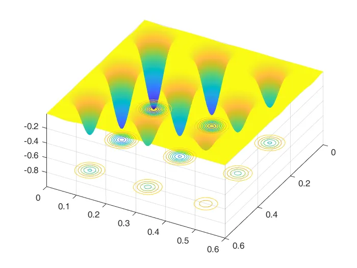
        surfc(X,Y,-f);
    % then To remove the lines produced by the mesh grid
        shading interp  
        %tital of graph 
        title('local maxima and global maxima')

out put figure :-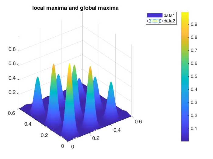

process of the program :-

% we start clear all, close all , clc .

%WE WILL PROVIDING THE SEARCH SPACE FOR THE FUNCTION

%Number of itreation for which the function will evaluate the fitness

%% WE WILL CREATING THE SURFACE PLOT OF STALAGEMITE FUNCTION

in the urface plot we used for loop and for loop or function formula

%now values of function in given search space

% then generating the surface

% then To remove the lines produced by the mesh grid

%tital of graph

for study 1

%% FOR STATISTICAL BEHAVIOUR (UNBOUNDED)

%calculating the study time through tic and toc command

%calculating the optimized value of the function

at this pont we used for loop ,and again for loop and function .

%at each iteration

%displaying the time taken to evaluate

% PLOTING THE GRAPH AND OPEN THE FIGURE WINDO

for study 2

%% STATISTICAL BEHAVIOUR (BOUNDED)

%calculating the study time through tic and toc command

%calculating the optimized value of the function

[inputs,fopt(j)]=ga(@stalagmite_func,2,[],[],[],[],[0;0],[1;1]);

%at each iteration with boundation

%PLOTTING for figure(2)

for study 3

%% MODIFYING THE NUMBER OF POPULATION

%increaing the sixe of population by usingoptimoptions function

used for loop and function

[inputs,fopt(k)]=ga(@stalagmite_func,2,[],[],[],[],[0;0],[1;1],[],[],options);

study3 we make plot and open the figure windo .

second code

function [stalagmite] = stalagmite_func(input_vector)
x = input_vector (1) 
y = input_vector (2)
f1_x = (sin(5.1*pi * x +0.5)).^6;
f2_y = (sin(5.1*pi * y +0.5)).^6;
f3_x = exp((-4*0.6931).*(x-0.0667)^2/(0.64));
f4_y = exp((-4*0.6931).*(y-0.0667)^2/(0.64));
stalagmite = (f1_x.*f2_y.*f3_x.*f4_y)
end



clear all
close all
clc

%% WE WILL PROVIDING THE SEARCH SPACE FOR THE FUNCTION

    x=linspace(0,0.6,150);
    y=linspace(0,0.6,150);
    [X,Y]=meshgrid(x,y);

 % Number of itreation for which the function will evaluate the fitness or
 % 50 times run the program .
    num_cases=50;


%% WE WILL CREATING THE SURFACE PLOT OF STALAGEMITE FUNCTION

     for i=1:length(X)
         for j=1:length(Y)
             input_vector(1)=X(i,j);
             input_vector(2)=Y(i,j);
             % Now values of function in given search space 
             f(i,j)=stalagmite_func(input_vector);   
         end
     end
  %generating the surface
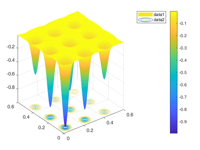
        surfc(X,Y,-f);  
  %To remove the lines produced by the mesh grid
        shading interp     
       
        
       
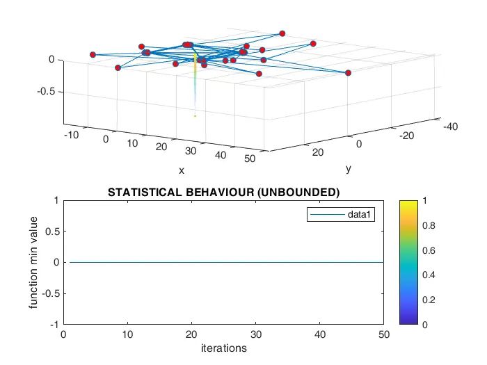
%% FOR STATISTICAL BEHAVIOUR (UNBOUNDED)        
%calculating the study time through tic and toc command        
tic                            
for i=1:num_cases
     %calculating the optimized value of the function 
        [inputs,fopt(i)]=ga(@stalagmite_func,2);
        %at each iteration
        xopt(i)=inputs(1);        
        yopt(i)=inputs(2);
    
end
 %displaying the time taken to evaluate
study1_time=toc   
    
        % PLOTING THE GRAPH AND OPEN THE FIGURE WINDO
        figure(1)

        subplot(2,1,1)

        surfc(X,Y,-f);      
        hold on
        shading interp
        plot3(xopt,yopt,-fopt,'marker','o','markersize',5,'markerfacecolor','r');
        xlabel('x');
        ylabel('y');
        grid on
        subplot(2,1,2)
        plot(-fopt);
        xlabel('iterations')
        ylabel('function min value')
        title('STATISTICAL BEHAVIOUR (UNBOUNDED)')
        
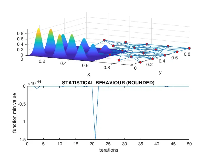
%% STATISTICAL BEHAVIOUR (BOUNDED)
%calculating the study time through tic and toc command
tic                                
 for j=1:num_cases
    %calculating the optimized value of the function  
        [inputs,fopt(j)]=ga(@stalagmite_func,2,[],[],[],[],[0;0],[1;1]); 
    %at each iteration with boundation
        xopt(j)=inputs(1);                                            
        yopt(j)=inputs(2);
    
 end
study2_time=toc
    
    %PLOTTING
    figure(2)
    
    subplot(2,1,1)
    hold on
    surfc(X,Y,-f)
    shading interp
    plot3(xopt,yopt,-fopt,'marker','o','markersize',5,'markerfacecolor','r');
    xlabel('x');
    ylabel('y');
    grid on
    subplot(2,1,2)
    plot(-fopt);
    xlabel('iterations')
    ylabel('function min value')
    title('STATISTICAL BEHAVIOUR (BOUNDED)')
   
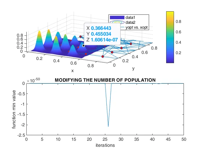
%% MODIFYING THE NUMBER OF POPULATION 
%increaing the sixe of population by usingoptimoptions function    
 options=optimoptions('ga','populationsize',400) 
 
 tic                                                    
for k=1:num_cases
    
    [inputs,fopt(k)]=ga(@stalagmite_func,2,[],[],[],[],[0;0],[1;1],[],[],options);
     xopt(k)=inputs(1);
     yopt(k)=inputs(2);         
     
end
study3_time=toc
    
    %PLOTTING
    figure(3)
    
    subplot(2,1,1)
    hold on
    surfc(X,Y,-f)
    shading interp
    plot3(xopt,yopt,-fopt,'marker','o','markersize',5,'markerfacecolor','r');
    xlabel('x');
    ylabel('y');
    grid on
    subplot(2,1,2)
    plot(-fopt);
    xlabel('iterations')
    ylabel('function min value')
    title(' MODIFYING THE NUMBER OF POPULATION ')

output figure :-

Week 4.1 - Genetic Algorithm

Ship work like this
in your own course.

Talk to a career counsellor

Ship work like thisin your own course.

Talk to a career counsellor

Ship work like this
in your own course.