Week 3 - Solving second order ODEs

• INTRODUCTION
• SIMPAL HARMONIC MOTION FOLLOW BY THE PENDULAM
• MOVEMENT OF PENDULAM DEPENDS ON NEWTON 2ND LOW
• SO THAT WE CAN WRITE DOWN A SECOND ORDER ORDINARY DIFFERENTIAL QUATION
• (d^2 ϴ)/(dt^2 )+b/(m ) dϴ/dt+g/l sinϴ=0 (this is the formula of equation of motion )

(d^2 ϴ)/(dt^2 )+b/(m ) dϴ/dt+g/l sinϴ=0 (this is the formula of equation of motion )

In the above equation

• G=gravity in M/s^2
• L=length of the pendulum in the meter.
• M=mass of the ball in kg
• B=damping coefficient.
• Since the given function is in the second order differential

Equation we will convert into first order to solve the ode.

• Let ϴ=ϴ1
• dθ1/dt=θ2

(dθ^2)/(dt^2 )=dθ2/dt

INPUT

• L=1 meters
• M=1kg
• B=0.05
• G=9.81m/s^2
• Time span =0-20 second
• Angular displacement =0
• Angular velocity = 3 rad/sec^2 at a time t=0

DETAIS OF EXPLANATION

• In the matlab first step is input the all parameters of the instrument and the know about pendulum position are fed.
• Then the use the ode45 which is in built function in matlab in this function we use with constant theta t and angular function is used which is defined separately in function program .
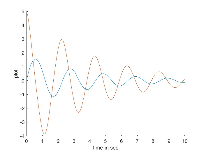
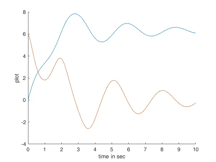
• In the next step result of solved ode is plotted with respect to time using plot command.
• Now we can use forloop for create animation .
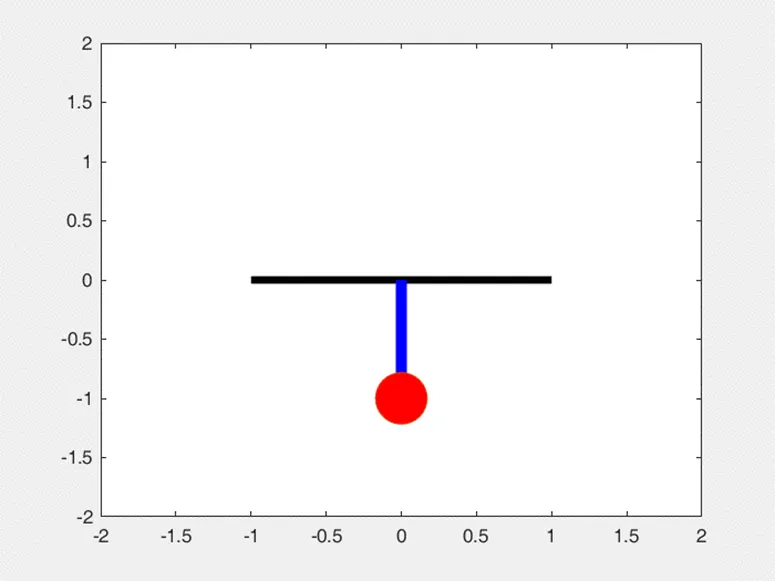
• Then the plot command is used to plot pendulum string and bob.
• Movie command use at last.

OUTPUT ANIMATION

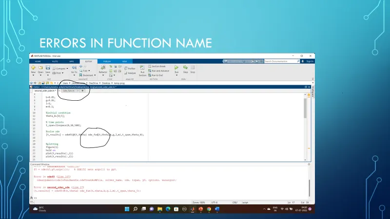
ERRORS AND RESOLVE

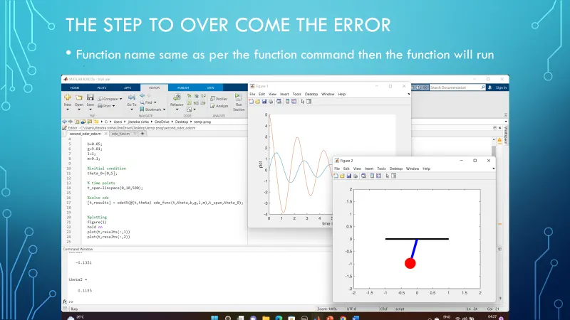
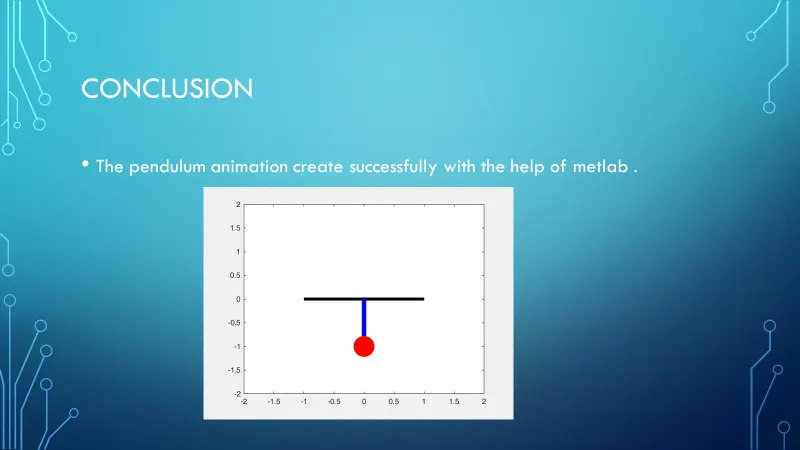
YOUTUBE LINK ANIMATION OF PENDULUM

https://youtu.be/DEqwuN8VVow

KINDLY LIKE SHEAR AND SUBSCRIB

clear all
close all 
clc

b=0.05;
g=9.81;
l=1;
m=0.1;

%initial condition
theta_0=[0;5];

% time points
t_span=linspace(0,10,500);

%solve ode
[t,results] = ode45(@(t,theta) ode_func(t,theta,b,g,l,m),t_span,theta_0);


%plotting
figure(1)
hold on
plot(t,results(:,1))
plot(t,results(:,2))

ylabel('plot')
xlabel('time')
xlabel('time in sec')

%iteration using for loop to create animation of simple pendulum

ct=1;

theta_1=results (:,1);
for i =1:length (results(:,1))

    %initial co-ordinates
    x_start=0;
    y_start=0;
    theta_2=theta_1(i);

    %final co-ordinates
    x_end =1*sin(theta_2);
    y_end =-1*cos(theta_2);

    %plotindg for animation
    figure(2)
    %base of pendulum 
    plot([-1,1],[0,0],'linewidth',4,'Color','black')
    hold on
    %string of pendulum
    line([x_start x_end],[y_start y_end],'linewidth',6,'color','b')
    hold on
    %bob of pendulum
    plot(x_end,y_end,'marker','o','markersize',28,'markerfacecolor','r')
    axis([-2 2 -2 2])
    pause (0.05)
    hold off
    M(ct)= getframe(gcf);
    ct=ct+1;
end  
 %animation 
 movie(M)
 videofile = VideoWriter('second_oder_ode','uncompressed AVI');
 open(videofile)
 writeVideo(videofile,M)
 close(videofile)

function[dtheta_dt]=ode_func(t,theta,b,g,l,m)

theta1=theta(1)
theta2=theta(2)
dtheta1_dt=theta2;
dtheta2_dt=-(b/m)*theta2-(g/l)*sin(theta1);
dtheta_dt=[dtheta1_dt;dtheta2_dt];

end