Week 4.1 - Genetic Algorithm

Here iam attaching the codes for the genetic algorithm:

%challenge in genetica algorithm using stalagamite function
clear all;
close all;
clc

%defining our search space
x = linspace(0,0.6,150);
y = linspace(0,0.6,150);
num_cases=50;


%creating a 2D mesh
[xx,yy] = meshgrid(x, y);
for i = 1 : length(xx)
    for j = 1 : length(yy)
    input_vector(1)=xx(i,j);
    input_vector(2)=yy(i,j);
    f(i,j) = stalagamite(input_vector);
    end
end

surfc(xx,yy,-f);
shading interp
tic
% Case 1 - statistical behaviour

for i = 1 : num_cases
    [inputs, fopt(i)] = ga(@stalagamite, 2);
    xopt(i) = inputs(1);
    yopt(i) = inputs (2);
end
case_1_time = toc

figure(2)
subplot(2, 1, 1);
hold on
surfc(xx,yy,-f);
shading interp
plot3(xopt, yopt,-fopt, 'marker','o','MarkerSize',5,'MarkerFaceColor','r')
title('unbounded inputs')
subplot(2,1,2)
plot(-fopt)
xlabel('iterations')
ylabel('function maximum')

%case_2 finding the lower and upper bounds

for i = 1 : num_cases
    [inputs, fopt(i)] = ga(@stalagamite,2,[],[],[],[], [0;0],[0.6; 0.6]);
    xopt(i) = inputs(1);
    yopt(i) = inputs (2);
end
case_2_time = toc

figure(3)
subplot(2, 1, 1);
hold on
surfc(xx,yy,-f);
shading interp
plot3(xopt, yopt,-fopt, 'marker','o','MarkerSize',5,'MarkerFaceColor','r')
title('upper and lower bounds')
subplot(2,1,2)
plot(-fopt)
xlabel('iterations')
ylabel('function maximum')

%Case 3 increasing ga itrations
options = optimoptions('ga');
options = optimoptions(options,'PopulationSize',200);

for i = 1 : num_cases
    [inputs, fopt(i)] = ga(@stalagamite,2,[],[],[],[], [0;0],[0.6; 0.6],[],[],options);
    xopt(i) = inputs(1);
    yopt(i) = inputs (2);
end
case_3_time = toc

figure(4)
subplot(2, 1, 1);
hold on
surfc(xx,yy,-f);
shading interp
plot3(xopt, yopt,-fopt, 'marker','o','MarkerSize',5,'MarkerFaceColor','r')
title('Bounded inputs with modified population size')
subplot(2,1,2)
plot(-fopt)
xlabel('iterations')
ylabel('function maximum')

Here iam attaching the plots what i got

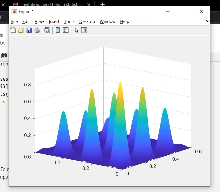
This is the plot i got for the first case

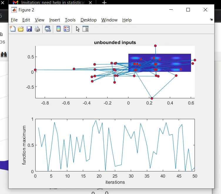
This is the plot i got for the Second case with the upper and lower bounds

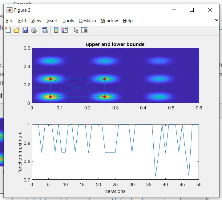
This is the plot i got for the Third case

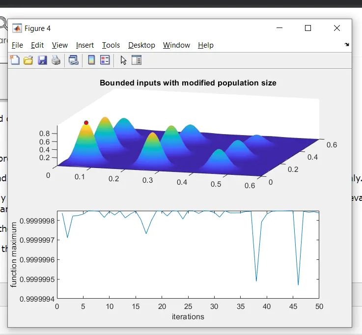
Here is the explaination for the program genetic algorithm

1. First i had entered the title and then i started with the code clear all close all and clc to start the program freshly.

2. Then i had entered the x and y values using the linspace command. then i have entered num cases. this is to evaluvate the ge algorithm what we did. It nearly mutes the x and y values when in the case study.

3. creating the 2d meash using the command mesh grid

4. then the for loop is started in this for loop we had given a two inputs as i and j. In i we taken a xx as an input vector1. In i we taken a yy as an input vector2. By using the call function we will describe the f value.

5. in the function command we have been taken the name as stalagamite and this fuction gives the f value by the following equation.

f(x, y) = f1x*f2x*f1y*f2y

6. By using this equation and the sub equation we could find the f value that is called as global minima. In this we can use the inverse form to find the global minima.

7. And in the ploting side xx,yy,-f to get the graph.

8. shading inturp is the command which is used to remove the grid lines in the surf plot we got. this command is to get the smooth surface.

9. By this codes we got the global maxima.

STALAGMITE :

It is the function which would find the global maxima

GENETIC ALGORITHM:

It is the algorithm which is used to find the global minima. Genitic algorithm is one of the optimization process.

It is based on the principle of the principle of population and natural selection.

It is used to solve the optimization problems in research and in machine learning.

***Then the case study 1 is to see the statistical behaviour

10. In this case study i had given a for loop to get the iterations for the num cases inthis it doesn't know about the x and y variables upper and lower limits.

11. In this the values get the xopt yopt and fopt to see the statistical behavior of GA.

12. In this the total study time is calculated by the command tic toc

13. in the ploting i was incerted the subplot command to see the two plots in the same figure window.

14. In this i got a two plots with various values and my x and y values was not get to the limits. It was exceeding the limits what i gave previously

***Then the case study 2 is to done with the upper and lower bounds.

15. In case study 2 the ga code which used is x = ga(fun,nvars,A,b,Aeq,beq,lb,ub) defines a set of lower and upper bounds on the design variables, x, so that a solution is found in the range lb ≤ x ≤ ub. (Set Aeq=[] and beq=[] if no linear equalities exist.) by this i had given a empty square brackets for the unkonwn values and proceded with the lower and upper boundaries of x and y.

16. after that the same code is to written for plotting section.

17. In this the time taken to finish the case study takes usual long when it compared to the case study 1.

18. in this the value set as the upper and lower boundries was reflected in the graph and it was found the best values

***Then the case study 3 is to done for the optimisation with the options command.

19. In case study 3 Global Optimasation is used for the best results in this the number of population size was increased and the number of iterations was gone high that's why the cyle time of this case study 3 time was huge when it compared to the both of the cases.

20. It was done by this sintax x = ga(fun,nvars,A,b,Aeq,beq,lb,ub,nonlcon,intcon,options) . In that the options i given the increased population size about to 200.

21. In this it gives the highest and lowest values of the x and y

22. The rest of the plotting command were given as same as the above case studies.

23. In this the value of x is 0.999