Week 4.1 - Genetic Algorithm

AIM: Write a code in MATLAB to optimize the stalagmite function and find the Global Maxima of the function.

Introduction:Genetic Algorithm (GA) is a search-based optimization technique based on the principles of Genetics and Natural Selection. It is frequently used to find optimal or near-optimal solutions to difficult problems which otherwise would take a lifetime to solve. It is frequently used to solve optimization problems, in research, and in machine learning

Objective:

• To Understand the concept of genetic algorithm
• To Understand the syntax “ga” in MATLAB
• To find the Global Maxima of the stalagmite function in MATLAB

MATLAB PROGRAM:

clear all
close all
clc

% Defining Our Search Space
x = linspace(0,0.6,150);
y = linspace(0,0.6,150);
num_cases = 50;         % no of itration

% Creating a 2Dimensional mesh
[xx ,yy] = meshgrid(x,y);

% Evaluating the Stalagmite Function
for i = 1:length(xx)
    for j = 1:length(yy)
        input_vector(1)=xx(i,j);
        input_vector(2)=yy(i,j);
        input_vector=[input_vector(1),input_vector(2)];
        GA(i,j) = stalagmite(input_vector);               

    end
end


% Study-1 | Statistical Behaviour | In Unbounded condition

tic                                     %tic_toc command for calculating the itration time                  
for i = 1:num_cases
        [input, GA_opt(i)] = ga(@stalagmite,2);
        xopt(i) = input(1);
        yopt(i) = input(2);
end

study_1_time = toc

%Plotting the Graph
figure(1) 
subplot(2,1,1)
hold on
surfc(x,y,-GA)
shading interp
plot3(xopt,yopt,-GA_opt,'marker','o','markersize',5,'markerfacecolor','r')
title('Unbounded inputs')
subplot(2,1,2)
plot(-GA_opt)
xlabel('Iteration')
ylabel('Function Minimum')


% Study-2 | Statistical behaviour - with upper & lower bounds

tic                                       
for i = 1:num_cases
    [input, GA_opt(i)] = ga(@stalagmite,2,[],[],[],[],[0;0],[1;1]);
        xopt(i) = input(1);
        yopt(i) = input(2);
end
study_2_time = toc

%Plotting the Graph
figure(2)
subplot(2,1,1)
hold on
surfc(x,y,-GA)
shading interp
plot3(xopt,yopt,-GA_opt,'marker','o','markersize',5,'markerfacecolor','r')
title('Bounded inputs')
subplot(2,1,2)
plot(-GA_opt)
xlabel('Iteration')
ylabel('Function Minium')


% Study-3 | Increasing GA Iterations

options = optimoptions('ga');                              %Calculating the optimum solution for 'ga' and save in options(variable)
options = optimoptions(options,'PopulationSize',240);      %increasing the size of population

tic                                                        
for i = 1:num_cases
    [input, GA_opt(i)] = ga(@stalagmite,2,[],[],[],[],[0;0],[1;1],[],[],options);
        xopt(i) = input(1);
        yopt(i) = input(2);
end
study_3_time = toc

%Plotting the Graph
figure(3)
subplot(2,1,1)
hold on
surfc(x,y,-GA)
shading interp
plot3(xopt,yopt,-GA_opt,'marker','o','markersize',5,'markerfacecolor','r')
title('Bounded inputs')
subplot(2,1,2)
plot(-GA_opt)
xlabel('Iteration')
ylabel('Function Minium')

• MATLAB program for the function.

function [GA] = stalagmite(input_vector)

x=input_vector(1);
y=input_vector(2);


term1 = pi*5.1*x;
term2 = pi*5.1*y;
term3 = ((x-0.0667)^2/0.64);
term4 = ((y-0.0667)^2/0.64);
term5 = (-4)*log(2);

xf1 = (sin(term1 + 0.5)).^6;

yf1 = (sin(term2 + 0.5)).^6;

xf2 = exp(term5*term3);

yf2 = exp(term5*term4);



GA=-(xf1*yf1*xf2*yf2);

end

Procedure:

Step 1- Start with usual Clear and closing command to clear memory. than defines the search space with 2 variable x & y. For that, creates 1-dimensional array for x,y & use linspace command to provide 150 value between 0 to 0.6.
After that I creates 2-dimensional array based on our 1-dimension array

Step 2- In next step, by using ‘for loop’, I define the Than I am creating an array called input_vector1, input_vector2 (row vectors) for each value of x,y and save these value in

input_vector.

Step 3- Now, to calculate maxima, I am typing a new function in
@stalagmite, by using the below formula-

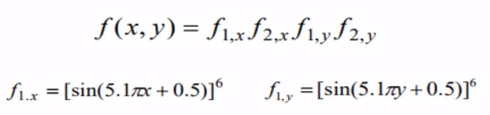
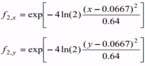
And stored its value in ‘GA’ Function.

Than this function, is called in for loop & passing the number of variable as input. So, that ‘for loop’ will generate the data for plot.

Step 4

1.Statistical Behaviour

After creating x,y variable(input variable),
as it does not define the search space for ‘ga’, ‘ga’ does not know its actual space and the value for x,y go beyond or below to 0.6 or 0.

For that I use num_cases=50, means I am going to run it 50 times.

Step a- I use ‘for loop’ and run the code from 1 to 50 times.
After that I call ga & use the new function which I created @stalagmite, pass 2 variable as input and store the output in GA_opt.
And than I store the value of ‘x &y’ in ‘xopt & yopt’

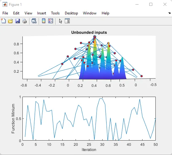
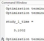
Step b- Now to visualize my output, i use surface command(surfc), shading command(shading interp) is used to get smooth plot(without grid lines). in new figure window(figure1), I also use tic-toc command to calculate the time taken for evaluation. I use subplot command for multiple plotting,
1^st plot to show stalagmite function, and plotting the minimum value that ‘ga’ trying to predict, over 50 studies.
2^nd plot for showing the number of iteration at x-axis and during each iteration value changes which represents as Function maxima on y-axis.

Result:

Command WIndow:

Step 5

2.Statistical Behaviour(with upper & lower bound)

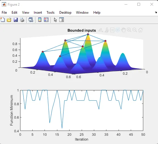
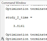
Step a- In this study, I setup the bound condition for the variables x&y, as it is going above & below the 0 & 0.6.

By using syntax ‘ga’ I am giving x&y the upper limit and lower limit to 0 to 1. I a doing so, because in previous study, it was observed from the graph that the optimum output lies all over the graph, so make it more clear and optimum, I am applying the boundary condition.

Results:

3.Increasing GA Iterations:

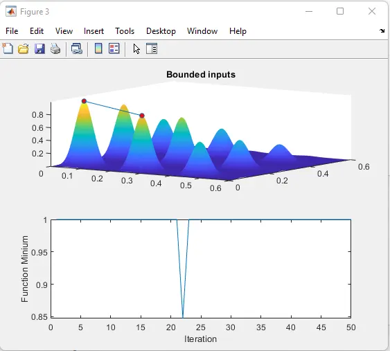
Step a- In addition with specifying bounds, I am also increasing initial population size. If population size is too small, we cannot find the global maxima, but we can find only local maxmia, which happens in study2.
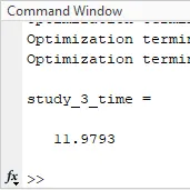
Following the same procedure as in study-2, and increase the population size to 240 and applying the constraint ‘optimoptions’ and save its values in variable ‘options’ to allow the ga to predict the optimum solution from 240 population size.

And plot graph for visual result

Result:

Based on the research, answer for following questions are;

Stopping criteria-
When there has been no improvement in the population for X iterations.

• When we reach an absolute number of generations.
• When the objective function value has reached a certain pre-defined value.

Syntax for ga- ga(@stalagmite,2,[ ],[ ],[ ],[ ],[0;0],[1;1],[ ],[ ],options)
ga(fun,nvars,A,b,Aeq,beq,lb,ub,nonlcon,options)

ga - To find the minimum of function using Genetic Algorithm
fun - finds a local minimum to function
nvars - number of variables.
A - Linear Inequality Constraints,specified as a real matrix
b - Linear Inequality Constraints,specified as a real vector
Aeq - Linear equality Constraints,specified as a real matrix
beq - Linear equality Constraints,specified as a real matrix
lb - Lower Bound
ub- Upper Bound
nonlcon - Nonlinear Constraints, specified as function handle
options- Optimization options, specified as the output

Significance of running multiple iterations -
We do Multiple iteration is to get the Global maxima in desired range. The main motive of doing so is to get the only 1 desired optimum output which is required for given problem.