Week 3 - Solving second order ODEs

Program to slove second order ODE:

                An ordinary differential equation (ODE) is a differential equation containing one or more functions of one indipendent variable and the derivatives of those functions. The ODE equation is shown below.

`(d^2theta)/dt^2 + b/m (d theta)/dt + sin theta = 0`

Function code for the ODE:

% function program to solve the ODE
function [dtheta_dt] = ode_func(t, theta,b,g,l,m)
theta1 = theta(1)
theta2 = theta(2)
dtheta1_dt = theta2
dtheta2_dt = -(b/m)*theta2 - (g/l)*sin(theta1)
dtheta_dt = [dtheta1_dt; dtheta2_dt]
end

Code for solving the ODE:

% Solving second order ODE of a penedulum
clear all 
close all
clc

% damping coefficient
b = 0.05 ;

% gravity (m/s^2)
g = 9.81;

% length of the spring (m)
 l = 1  ;

 % mass of the bob (kg)
 m = 0.1 ;

% initial condition, angular displacement is 0 and angular velocity is 5
theta_0 = [0;5];

% time span, Pendulum oscillates between 0-20 seconds
t_span = linspace(0,20,500);

% solving ODE 
[t,results] = ode45(@(t,theta)ode_func(t,theta, b,g,l,m),t_span,theta_0);

%Plotting
figure(1) 
hold on 
plot(t,results(:,1))
plot(t,results(:,2)) 
title('Damped Harmonic motion of a Pendulum')
legend('Angular displacement', 'Angular velocity')
xlabel('Time (seconds)')
ylabel('Plot') 

% For loop (Before starting the for loop, a counter value was defined)
ct = 1;
for i = 1:length(results(:,1)) 
    x_start =0;
    y_start =0;
    x_end = l*sin(results(i,1));
    y_end = -l*cos(results(i,1));

% plotting the animation
figure(2) 
plot([-1 1], [0,0], 'linewidth', 5) 
hold on
plot([x_start x_end],[y_start y_end],'LineWidth',3)
hold on

plot(x_end,y_end,'o', 'MarkerSize',20,'MarkerFaceColor','y')
title('Animation of pendulum')
axis([-1.5 1.5 -1.5 1])
pause(0.03)
hold off

M(ct) = getframe(gcf);
ct = ct+1;
end

% Animation of pendulum
movie(M)
videofile=VideoWriter('pendulum animation.avi', 'Uncompressed AVI');
open(videofile)
writeVideo(videofile,M)
close(videofile)

Code explanation:

•  Start with clear all, close all and clc commands since,
• Clear all - removes data from the workspace, freeing up system memory.
• Close all-deletes the current figure or the specified figure.
• clc - clears all input and output from the Command Window display, giving you a "clear window".
• Define the inputs and variables. The damping coefficient, gravity, length of the spring and mass of the bob have all been defined.
• Define the initial conditions, the angular displacement and angular velocity have been defined. Timespan has also been defined.
• Solve the ODE, Ode45 was used, it is a function in Matlab that solves ordinary or partial differential equations using a numerical method. The numerical method in question here is the 4th order Runge kutta method. The function ode45 takes 3 inputs. The 3 inputs are the function to be integrated, the time span and the initial conditions. [t, results] means that the results that have been calculated with respect to time.
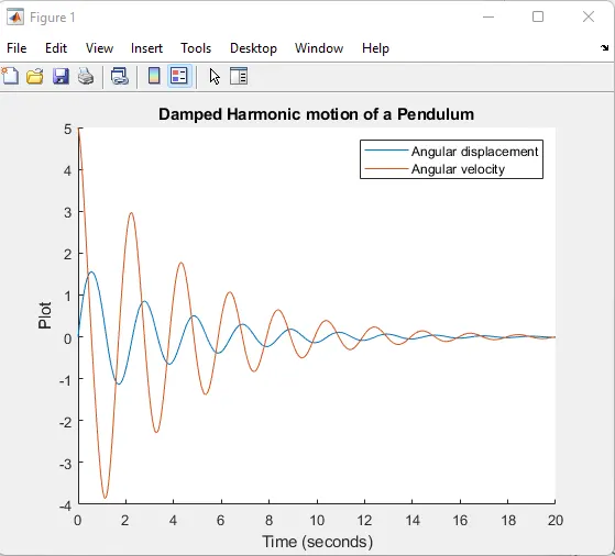
• After calculating the results, a graph has to be plotted, the graph contained two plots. One for angular displacement with respect to time and one for angular velocity with respect for time. The legend for the graph and the axis' labels have been defined. Figure 5 shows the graph obtained.

• The second part of the code is to establish a for loop.

• A counter loop was added before the For loop. T

• he start and endpoints for x and y-axis have been defined.

• The loop is used where all the values of timespan are assigned to a variable i one at a time.

• The coordinates of [ xo x1 yo y1] and their corresponding relations are entered to form a 'string' of the pendulum.

• Markersize command was used to form the bob of the pendulum.

• A pause command was used for pausing the command for a certain time, for this project a pause of 0.03 s was used.

• The M command was used to capture the current frame every time the for loop runs.

• The final step of the loop is to add a '+1' to the ct variable, this will increment the frame every time the for loop run.

• End command was used for the plot and for the 'for loop' to stop both from running.

• The final step of the code is to create a movie of the animation, so the movie command was used.

• The Video Writer command was used to assign the video format, for this project .avi was used as the format.

• The open command was used to open the video.

• writevideo command was used to write the video with plot frames.

• Finally, the close command was used to close the video file.

Graph:

Animation video link:

Click here