Week 4.1 - Genetic Algorithm

Objective:

To write a code in MATLAB to optimize the stalagmite function and find the global maxima of the function.

Genetic algorithm:

• The genetic algorithm is a method for solving both constrained and unconstrained optimization problems that are based on natural selection, the process that drives biological evolution.
• The genetic algorithm repeatedly modifies a population of individual solutions.
• At each step, the genetic algorithm selects individuals from the current population to be parents and uses them to produce the children for the next generation.
• Over successive generations, the population "evolves" toward an optimal solution.
• We can apply the genetic algorithm to solve a variety of optimization problems that are not well suited for standard optimization algorithms, including problems in which the objective function is discontinuous, nondifferentiable, stochastic, or highly nonlinear.
• The genetic algorithm can address mixed integer programming problems, where some components are restricted to integer-valued.

The GA syntax in Matlab is given by :

x=ga(fun,nvars,A,B.Aeq.Beq,LB,UB.nonlcon,intcon,options)

Here,

• fun = objective function
• nvars = number of variables
• A and B = subject to linear inequalities of the form A*x <=B
• Aeq and Beq = subject to linear equalities of the form A*x = B
• LB = lower bound
• UB = upper bound
• nonlcon = non linear inequalities
• intcon = integer constrained
• options = helps to add contraint tolerance by increasing the population size

Function code:

function [f] = stalagmite(input)
x = input(1);
y = input(2);

f1_x = (sin((5.1*pi*x)+0.5)).^6;
f1_y = (sin((5.1*pi*y)+0.5)).^6;

f2_x = exp(((-4*log(2))*(x-0.0667).^2)/0.64);
f2_y = exp(((-4*log(2))*(y-0.0667).^2)/0.64);

[f] = -(f1_x.*f1_y.*f2_x.*f2_y);
end

Main code:

clear all
close all
clc

%Defining our search space
x = linspace(0,0.6,150);
y = linspace(0,0.6,150);
[xx,yy] = meshgrid(x,y); 
num_cases = 80 ;

%calling stalagmite function 
for i = 1:length(xx)
    for j = 1:length(yy)
        input(1) = xx(i,j);
        input(2) = yy(i,j);
        f(i,j) = stalagmite(input);
    end
end

%Study 1 - Statistical behavior
tic
for i=1:num_cases
    [inputs, fopt(i)] = ga(@stalagmite,2);
    xopt(i) = inputs(1);
   yopt(i) = inputs(2);
 
end

study1_time = toc
 
figure(1)
subplot(2,1,1)
hold on
surfc(xx,yy,f)
shading interp
title('Unbound inputs')
xlabel('X values')
ylabel('Y values')
plot3(xopt,yopt,fopt,'marker','o','markersize',5,'markerfacecolor','r')

subplot(2,1,2)
plot(fopt)
xlabel('Iterations')
ylabel('Function maximum')

%Study 2 - Statistical behavior with upper and lower bounds
tic
for i=1:num_cases
    [inputs, fopt(i)] = ga(@stalagmite,2,[],[],[],[],[0;0],[0.6;0.6]);
    xopt(i) = inputs(1);
   yopt(i) = inputs(2);
end

 study2_time = toc
 
figure(2)
subplot(2,1,1)
hold on
surfc(xx,yy,f)
shading interp
title('Bounded inputs')
xlabel('X values')
ylabel('Y values')
plot3(xopt,yopt,fopt,'marker','o','markersize',5,'markerfacecolor','r')
subplot(2,1,2)
plot(fopt)
xlabel('Iterations')
ylabel('Function maximum')

%Study 3 - Increasing GA iterations
options = optimoptions('ga')
options = optimoptions(options,'populationSize',200)

tic
for i=1:num_cases
    [inputs, fopt(i)] = ga(@stalagmite,2,[],[],[],[],[0;0],[0.6;0.6],[],[],options);
    xopt(i) = inputs(1);
   yopt(i) = inputs(2);
end

 study3_time = toc
 
figure(3)
subplot(2,1,1)
hold on
surfc(xx,yy,f)
shading interp
xlabel('X values')
ylabel('Y values')
plot3(xopt,yopt,fopt,'marker','o','markersize',5,'markerfacecolor','r')
subplot(2,1,2)
plot(fopt)
xlabel('Iterations')
ylabel('Function maximum')

Code explanation:

• We are providing the inputs using linspace to define x and y.
• Next we define the Stalagmite_func.
• The loops are incorporated into the main code so that all the combinations of x and y values are taken in the stalagmite_func function.

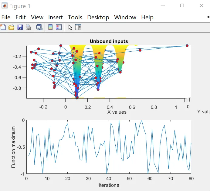
Study 1:

• There are no lower and upper limits in study 1 so Ga does not search space between 0 and 1.
• So that each time the program is executed different values is obtained.

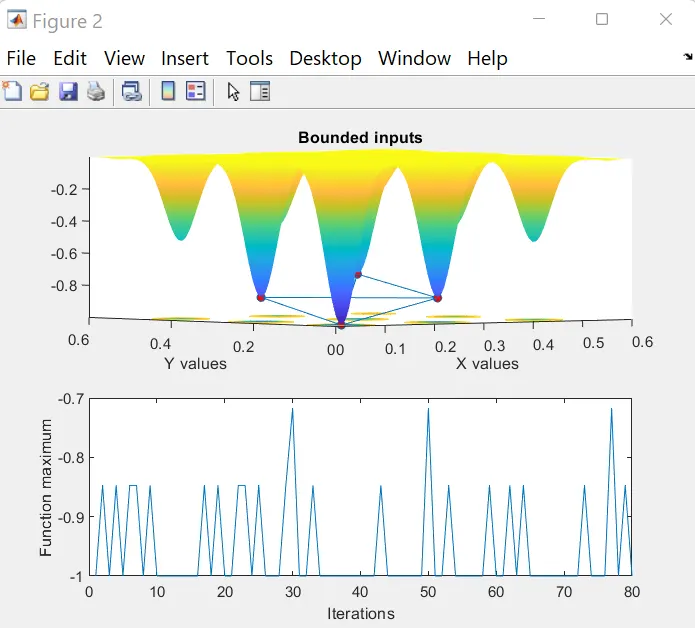
Study 2:

• The lower and upper limits are included in study 2.
• So, the maximum values obtained vary between -1 and -0.7.

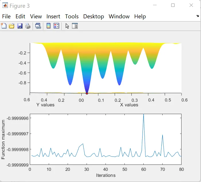
Study 3:

• Here the GA function is incorporated with lower and upper bounds along with the population size of 200.
• The global maximum obtained is accurate and is narrowed down to a value of -0.999999.

Result:

We have created a code in MATLAB to optimize the stalagmite function and find the global maxima of the function.