Week 4.1 - Genetic Algorithm

the funtion is carries as a outer funtion, the code for the funtion is

%stalagmite1 function coding

function [f]=stalagmite1(input)

x=input(1);
y=input(2);

f1x=(sin((5.1*pi*x)+0.5))^6;
f1y=(sin((5.1*pi*y)+0.5))^6;
f2x=exp(-4*log(2)*(((x-0.0667)^2)/0.64));
f2y=exp(-4*log(2)*(((y-0.0667)^2)/0.64));

f = -(f1x*f1y*f2x*f2y);
end

and the x and y values are meshgrid and made it as matrix form.

for i = 1:length(x)

    for j = 1:length(y)
        
        input(1)= xx(i,j);
        input(2)= yy(i,j);

        f(i,j) = stalagmite1(input);
    end

end

with the coding we have got the x,y,f values

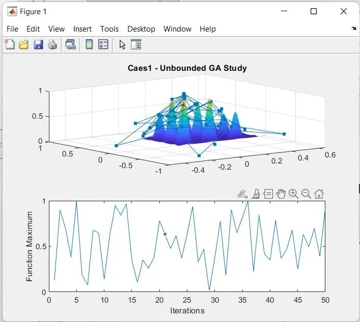
for Case-1

the condition is unbounded range so applying the whole range

ie in code is

%case 1 figure representation
figure(1)
subplot(2,1,1)
surf(x,y,-f)
shading interp
hold on

plot3(xopt,yopt,-fopt,'marker','.','markersize',10)
title('Caes1 - Unbounded GA Study')
subplot(2,1,2)

the surface plotting is done , we also need to plot the f-maximum vs iterations

%Plot between 'Iterations' and 'Function Maximum'
subplot(2,1,2)
plot(-fopt)    
xlabel('Iterations')
ylabel('Function Maximum')

hence the first figure forms as

Case-2

case 2 codition is to be in the range, hence we are providing the 0, 0.4 along x and y in the ga function, to form new fopt values

%case2 - bounded

for i = 1:50

    [input,fopt(i)]=ga(@stalagmite1,2,[],[],[],[],[0,0],[0.4,0.4]);

    xopt(i) = input(1);
    yopt(i) = input(2);

end

therefore the code for surface figure

%case 2 figure representation
figure(2)
subplot(2,1,1)
surf(x,y,-f)
shading interp
hold on

plot3(xopt,yopt,-fopt,'marker','.','markersize',10)
title('Case2 - Bounded GA Study')

for subplotting of the graph is

subplot(2,1,1)
%Plot between 'Iterations' and 'Function Maximum'
subplot(2,1,2)
plot(-fopt)    
xlabel('Iterations')
ylabel('Function Maximum')

and the figure forms as

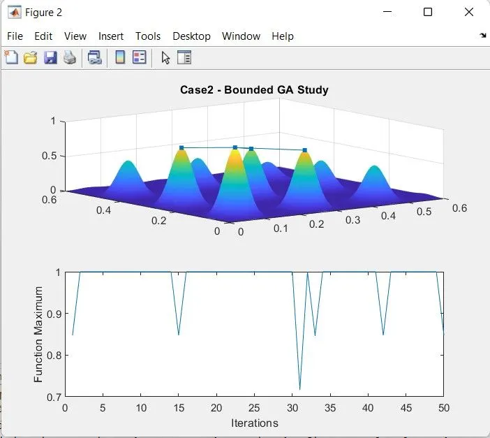
the case 2 is finished

Case 3

The case 3 condition is bounded range with population size

the population size is inputted with options within the Population function.

%assigning option
options = optimoptions('ga');
options = optimoptions(options,'PopulationSize',270);

using for loop to assign options in 50 iteration

for i = 1:50

    [input,fopt(i)]=ga(@stalagmite1,2,[],[],[],[],[0,0],[0.4,0.4],[],[],options);

    xopt(i) = input(1);
    yopt(i) = input(2);

end

then the values are taken to create surface plotting and plot of fmaximum vs iteration.

figure(3)
subplot(2,1,1)
surf(x,y,-f)
shading interp
hold on

plot3(xopt,yopt,-fopt,'marker','.','markersize',10)
title('Case3 - Bounded GA study with Population Size')

subplot(2,1,1)
%Plot between 'Iterations' and 'Function Maximum'
subplot(2,1,2)
plot(-fopt)    
xlabel('Iterations')
ylabel('Function Maximum')

the figure 3 becomes

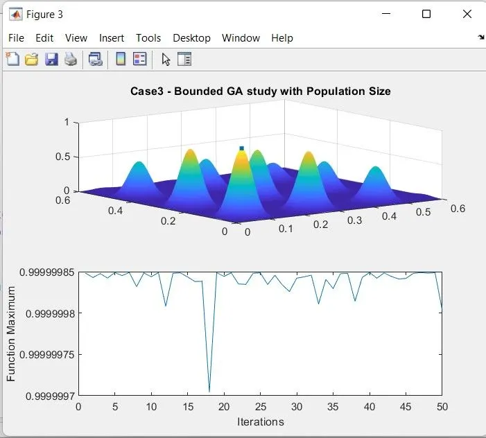
hence the plotting of 3 conditions are done.

the finddings are the plot of fmaximum vs iteration tells about the values becoming less deviative with 50 iteration

Full codes

Function code

%stalagmite1 function coding

function [f]=stalagmite1(input)

x=input(1);
y=input(2);

f1x=(sin((5.1*pi*x)+0.5))^6;
f1y=(sin((5.1*pi*y)+0.5))^6;
f2x=exp(-4*log(2)*(((x-0.0667)^2)/0.64));
f2y=exp(-4*log(2)*(((y-0.0667)^2)/0.64));

f = -(f1x*f1y*f2x*f2y);
end

Main code

clear all
close all
clc


%genetic algorithm

%defining input space
x= linspace(0,0.6,150);
y= linspace(0,0.6,150);

%mesh by meshgrid

[xx,yy] = meshgrid(x,y);

for i = 1:length(x)

    for j = 1:length(y)
        
        input(1)= xx(i,j);
        input(2)= yy(i,j);

        f(i,j) = stalagmite1(input);
    end

end



%case1 - unbounded

for i = 1:50

    [input,fopt(i)]=ga(@stalagmite1,2);

    xopt(i) = input(1);
    yopt(i) = input(2);

end

%case 1 figure representation
figure(1)
subplot(2,1,1)
surf(x,y,-f)
shading interp
hold on

plot3(xopt,yopt,-fopt,'marker','.','markersize',10)
title('Caes1 - Unbounded GA Study')
subplot(2,1,2)

%Plot between 'Iterations' and 'Function Maximum'
subplot(2,1,2)
plot(-fopt)    
xlabel('Iterations')
ylabel('Function Maximum')

%case2 - bounded

for i = 1:50

    [input,fopt(i)]=ga(@stalagmite1,2,[],[],[],[],[0,0],[0.4,0.4]);

    xopt(i) = input(1);
    yopt(i) = input(2);

end

%case 2 figure representation
figure(2)
subplot(2,1,1)
surf(x,y,-f)
shading interp
hold on

plot3(xopt,yopt,-fopt,'marker','.','markersize',10)
title('Case2 - Bounded GA Study')

subplot(2,1,1)
%Plot between 'Iterations' and 'Function Maximum'
subplot(2,1,2)
plot(-fopt)    
xlabel('Iterations')
ylabel('Function Maximum')



%case3 - bounded with population size

%assigning option
options = optimoptions('ga');
options = optimoptions(options,'PopulationSize',270);

for i = 1:50

    [input,fopt(i)]=ga(@stalagmite1,2,[],[],[],[],[0,0],[0.4,0.4],[],[],options);

    xopt(i) = input(1);
    yopt(i) = input(2);

end

figure(3)
subplot(2,1,1)
surf(x,y,-f)
shading interp
hold on

plot3(xopt,yopt,-fopt,'marker','.','markersize',10)
title('Case3 - Bounded GA study with Population Size')

subplot(2,1,1)
%Plot between 'Iterations' and 'Function Maximum'
subplot(2,1,2)
plot(-fopt)    
xlabel('Iterations')
ylabel('Function Maximum')

the code used in here are simple codes.

CONCLUTION:

Hence, the Aim of creating a code in MATLAB to optimise the stalagmite function and find the global maxima of the function.and plotting graphs for all 3 cases and for F maximum vs no. of iterations. is done successfully