Project 1 - Parsing NASA thermodynamic data
Project 1 - Parsing NASA thermodynamic data
AIM:
To load data and plot graph for cp, h s and to to find the molecular weight from the data provided in the file using MATLAB
OBJECTIVE:
- To load the data and assigning the variables
- Write a CODE to create CP,H,S diagram with respective to the T of the given data
- To find the Molecular weight and display it in the COMMAND WINDOW
EQUATIONS USED:
The formula used for calculating the thermodynamics
Here R is Universal Gas Constant and T is Temperature

where Cp is specific heat , H Enthalpy , S is Enthropy.
PROCEDURE:
To load the given data file Nasa Thermodynamic Data
the file is download and the path of the file is assignes as same as mathlab file, then the file is loaded using
%file reading

f1 = fopen('THERMO.dat','r');
the file is loading, the file is in the formate which look like this when open in window.
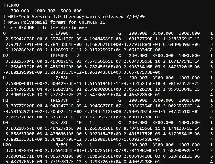
there fore the first 5 line are needed to be skipped , that is done with
%to skip the first 5 lines as they are heading in the document
for i= 1:5
    fgetl(f1);
end
now we get to the part of 53 parts or species details in 4 line format, so we apply a for loop in 1:53 as what all we do will be repeated for the 53 species that is
%Assigning for 53 species with for loop in 53 times
for k= 1:53
.
.
.
.
.
.
.
end
all the functions are carried out between these
THE CODE FOR ASSIGNING THE DATA
the first line is assigned by
%assigning the line as a
a = fgetl(f1);
Spliting the line
%spliting the string
b = strsplit(a,' ');
there for assigning the name of species.
%Assigning speciesname as first one in the line
speciesname = b{1}
then the data fot Temperature, the temp data is assigned as low_temp, high_temp, mid_temp order, so they are assigned as
%Assigning local temperature
% among the given data the temperature will be in the format
%(low_temp, high_temp, mid_temp) for all 53 species
low_temp = str2double(b{end-3});
high_temp = str2double(b{end-2});
mid_temp = str2double(b{end-1});
the 14 co efficients are assigned as
%extraxting the 14 coefficient

line1 = fgetl(f1);

pos = strfind(line1,'E');

a1 = str2double(line1(1:(pos(1)+3)));
a2 = str2double(line1((pos(1)+4):(pos(2)+3)));
a3 = str2double(line1((pos(2)+4):(pos(3)+3)));
a4 = str2double(line1((pos(3)+4):(pos(4)+3)));
a5 = str2double(line1((pos(4)+4):(pos(5)+3)));

line2 = fgetl(f1);

a6 = str2double(line2(1:(pos(1)+3)));
a7 = str2double(line2((pos(1)+4):(pos(2)+3)));
a8 = str2double(line2((pos(2)+4):(pos(3)+3)));
a9 = str2double(line2((pos(3)+4):(pos(4)+3)));
a10 = str2double(line2((pos(4)+4):(pos(5)+3)));

line3 = fgetl(f1);

a11 = str2double(line2(1:(pos(1)+3)));
a12 = str2double(line2((pos(1)+4):(pos(2)+3)));
a13 = str2double(line2((pos(2)+4):(pos(3)+3)));
a14 = str2double(line2((pos(3)+4):(pos(4)+3)));
the assigning parts are done .
- The calculation of Cp, H, S
the the calulations are done to plot the graph with temparature hence the T value is assigned with linspace function,
T = linspace(low_temp, high_temp,100);the data gives the low_temp and High_temp, values, the coeffcient given are in first 7 for high temparature and then 7 for low temparature.
the function to apply the temparatures are determine the region
for i = 1: length(T)

    if (T(i))<= mid_temp

        T1(i) = T(i);

    elseif (T(i))>= mid_temp

        T2(i) = T(i);

    end
end
then the high temp region and low temp region areassigned , as
ltr = T1;
d = length(ltr);
htr = T2((d+1):100);
R   = 8.314;
the calculations are done
     cp1 = (a1 + a2*htr + a3*htr.^2 + a4*htr.^3 + a5*htr.^4)*R;
     H1  = (a1 + (a2*htr)/2 + (a3*htr.^2)/3 + (a4*htr.^3)/4 + (a5*htr.^4)/5 + (a6./htr))*R.*htr;
     S1  = (a1*log(htr)+a2.*htr+(a3*htr.^2)/2+(a4*htr.^3)/3+(a5*htr.^4)/4+a7);

     cp2 = (a8 + a9*ltr + a10*ltr.^2 + a11*ltr.^3 + a12*ltr.^4)*R;
     H2  = (a8 + (a9*ltr)/2 + (a10*ltr.^2)/3 + (a11*ltr.^3)/4 + (a12*ltr.^4)/5 + (a13./ltr))*R.*ltr;
     S2  = (a8*log(ltr)+a9.*ltr+(a10*ltr.^2)/2+(a11*ltr.^3)/3+(a12*ltr.^4)/4+a14)*R;
then the parts are combine together
     CP = [cp1,cp2];
     H = [H1,H2];
S = [S1,S2];- Plotting graph and saving in the files
the plotting is done by simple plot command but a mkdir function is used before the plotting funtion and cd is used to close the funtion for saving data
     mkdir(['C:\Users\anis2\Downloads\nasa td\',speciesname]);

     figure(1)
     plot(T, CP)
     xlabel('Temperature')
     ylabel('Specific heat')
     title('Specific heat vs Temperature of',speciesname)

     figure(2)
     plot(T, H)
     xlabel('Temperature')
     ylabel('Enthalpy')
     title('Enthalpy vs Temperature of',speciesname)

     figure(3)
     plot(T, S)
     xlabel('Temperature')
     ylabel('Entropy')
     title('Entropy vs Temperature of',speciesname)


     cd(['C:\Users\anis2\Downloads\nasa td\',speciesname]);
     saveas(1,'Specific heat vs Temperature')
     saveas(2,'Enthalpy vs Temperature')
     saveas(3,'Entropy vs Temperature')
the plotting will be seen as
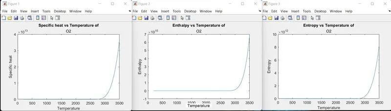
wil the x axis and y axis labels
- To find the molecular weight
the molecular weight function is carries out as a sperate function, with the code
function W = MW(speciesname)

%molecular weight

atoms = ['H','C','N','O','A'];
% mass to be allocated
mass = [1.0079 , 12.0107, 14.0067, 15.999, 39.948];

W=0;

for i = 1:length(speciesname)

    for j = 1:length(atoms)

        if strcmp(speciesname(i),atoms(j))
            W= W+ mass(j);
            position = j;
        end
    end
          number= str2num(speciesname(i));
          if (number>1)
              W = W + (mass(position)*(number - 1));
          end

end
and the cade in teh main code to call the function is
%To find Molecular Weight
Wm = MW(speciesname);
sprintf('Molecular Weight of %s : %.2f u',speciesname,Wm)
can be seen as
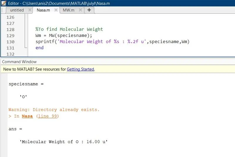
the for loop started in the first with k= 1:53 is end ed here to get the 53 species plottings and molecular weight in the commad window
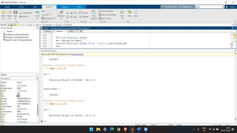
and the files are saved as

the graphs can be assessed , like for N2
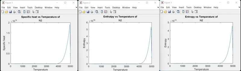
for CO2
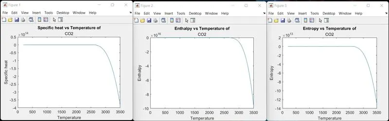
the full code is
clear all
close all
clc

%file reading

f1 = fopen('THERMO.dat','r');

%to skip the first 5 lines as they are heading in the document
for i= 1:5
    fgetl(f1);
end

%Assigning for 53 species with for loop in 53 times
for k= 1:53

%assigning the line as a
a = fgetl(f1);

%spliting the string
b = strsplit(a,' ');

%Assigning speciesname as first one in the line
speciesname = b{1}

%Assigning local temperature
% among the given data the temperature will be in the format
%(low_temp, high_temp, mid_temp) for all 53 species
low_temp = str2double(b{end-3});
high_temp = str2double(b{end-2});
mid_temp = str2double(b{end-1});


%extraxting the 14 coefficient

line1 = fgetl(f1);

pos = strfind(line1,'E');

a1 = str2double(line1(1:(pos(1)+3)));
a2 = str2double(line1((pos(1)+4):(pos(2)+3)));
a3 = str2double(line1((pos(2)+4):(pos(3)+3)));
a4 = str2double(line1((pos(3)+4):(pos(4)+3)));
a5 = str2double(line1((pos(4)+4):(pos(5)+3)));

line2 = fgetl(f1);

a6 = str2double(line2(1:(pos(1)+3)));
a7 = str2double(line2((pos(1)+4):(pos(2)+3)));
a8 = str2double(line2((pos(2)+4):(pos(3)+3)));
a9 = str2double(line2((pos(3)+4):(pos(4)+3)));
a10 = str2double(line2((pos(4)+4):(pos(5)+3)));

line3 = fgetl(f1);

a11 = str2double(line2(1:(pos(1)+3)));
a12 = str2double(line2((pos(1)+4):(pos(2)+3)));
a13 = str2double(line2((pos(2)+4):(pos(3)+3)));
a14 = str2double(line2((pos(3)+4):(pos(4)+3)));


%calculation of Cp, H, S

T = linspace(low_temp, high_temp,100);

for i = 1: length(T)

    if (T(i))<= mid_temp

        T1(i) = T(i);

    elseif (T(i))>= mid_temp

        T2(i) = T(i);

    end
end

ltr = T1;
d = length(ltr);
htr = T2((d+1):100);
R   = 8.314;


%for j = 1:length(T)
 %   if (T(j)<=mid_temp)

     cp1 = (a1 + a2*htr + a3*htr.^2 + a4*htr.^3 + a5*htr.^4)*R;
     H1  = (a1 + (a2*htr)/2 + (a3*htr.^2)/3 + (a4*htr.^3)/4 + (a5*htr.^4)/5 + (a6./htr))*R.*htr;
     S1  = (a1*log(htr)+a2.*htr+(a3*htr.^2)/2+(a4*htr.^3)/3+(a5*htr.^4)/4+a7);

     cp2 = (a8 + a9*ltr + a10*ltr.^2 + a11*ltr.^3 + a12*ltr.^4)*R;
     H2  = (a8 + (a9*ltr)/2 + (a10*ltr.^2)/3 + (a11*ltr.^3)/4 + (a12*ltr.^4)/5 + (a13./ltr))*R.*ltr;
     S2  = (a8*log(ltr)+a9.*ltr+(a10*ltr.^2)/2+(a11*ltr.^3)/3+(a12*ltr.^4)/4+a14)*R;

     CP = [cp1,cp2];
     H = [H1,H2];
     S = [S1,S2];

     mkdir(['C:\Users\anis2\Downloads\nasa td\',speciesname]);

     figure(1)
     plot(T, CP)
     xlabel('Temperature')
     ylabel('Specific heat')
     title('Specific heat vs Temperature of',speciesname)

     figure(2)
     plot(T, H)
     xlabel('Temperature')
     ylabel('Enthalpy')
     title('Enthalpy vs Temperature of',speciesname)

     figure(3)
     plot(T, S)
     xlabel('Temperature')
     ylabel('Entropy')
     title('Entropy vs Temperature of',speciesname)


     cd(['C:\Users\anis2\Downloads\nasa td\',speciesname]);
     saveas(1,'Specific heat vs Temperature')
     saveas(2,'Enthalpy vs Temperature')
     saveas(3,'Entropy vs Temperature')


%To find Molecular Weight
Wm = MW(speciesname);
sprintf('Molecular Weight of %s : %.2f u',speciesname,Wm)
end
CONCLUTION:
Hence, the Aim
- To load data
- Save the plotted graph for Cp, H, S
- to find the molecular weight
from the data provided in the file using MATLAB is done successfully
note:- the loading data to matlab and using data to apply or calculate in the function , its important to know about the string functions are its uses.