Week 3 - Solving second order ODEs

Solving a Second Order ODE and An Animation of Oscillation of Pendulum using MATLAB

AIM:

To solve a second order ODE that represents the equation of motion of a simple pendulum with damping and making an Animation of the movement of the pendulum using MATLAB

OBJECTIVE:

• Write a CODE to solve the Second order ODE of pendulum
• To make the Animation of the movement of pendulum

GIVEN EQUATION AND INPUTS:

The given second order equation is

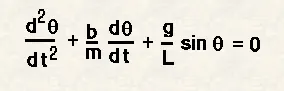
Also given

gravity g in m/s2

g= 9.81

Length l in m

l= 1

Mass of the ball in kg

m= 1

Damping coefficient

b=0.05

PROCEDURE:

• SOLVING THE GIVEN SECOND ORDER EQUATION.
• WE HAVE CHOOSEN THE ODE45 FUNCTION HENCE THE PROBLEM IS CONVERTED TO FIRST ORDER EQUATION

THE Process is carries out by another function

That given function is

(d^2(theta)/dt) + (b/m).(d(theta)/dt)+(g/l).sin(theta)=0

Sub theta1=theta

(d^2(theta1)/dt) + (b/m).(d(theta1)/dt)+(g/l).sin(theta1)=0

Sub theta2= (d(theta1)/dt)

Ie (d.(d(theta1)/dt)/dt) + (b/m).(d(theta1)/dt)+(g/l).sin(theta1)=0

(d .(theta2)/dt) + (b/m).( theta2)+(g/l).sin(theta1)=0

The equation is done with a derivation function

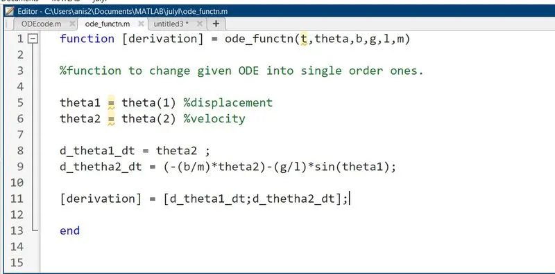
function [derivation] = ode_functn(t,theta,b,g,l,m)

%function to change given ODE into single order ones. 

theta1 = theta(1) %displacement
theta2 = theta(2) %velocity 

d_theta1_dt = theta2 ;
d_thetha2_dt = (-(b/m)*theta2)-(g/l)*sin(theta1);

[derivation] = [d_theta1_dt;d_thetha2_dt];

end

• ASSIGNING OTHER VALUES

The other values are

• THE ANGULAR DISPLACEMENT AND ANGULAR VELOCITY ARE FOUND BY

  [t,r] = ode45(@(t,theta) ode_functn(t,theta,b,g,l,m),t_span,theta_0);​

  then the Angular Displacement and Angular velocity are got in a matrix of 2 colum

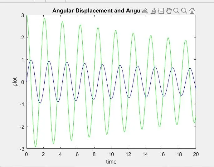
• %plotting of Angular Displacement and Angular velocity

  the plot function is used to plot the time vs Angular Displacement and Angular velocity graph

  figure(1)
  plot(t,r(:,1),"Color",'b')%Angular Displacement in blue
  hold on 
  plot(t,r(:,2),"Color",'g')%Angular velocity in green
  xlabel('time')
  ylabel('plot')
  title('Angular Displacement and Angular velocity')

  and the output is

  

  • THE PENDULUM ANIMATION

  The pedulum animation of done by plotting of pendulum movements, the pendulum movement frames

  the for loop is used for the function and the displacement values are assigned for the positioning and also for ploting the line the sine and cosine functions are used, as the pendulumis moving below or down side, the minus(-) is usedin from of the Yaxis term

  the code for animation teh getframe is used in side the loop

  %pendulam animation
  
  x0=0;
  y0=0;
  displacement_values = r(:,1);
  
  ct = 1;
  
  for i = 1:length(displacement_values)
  
      x1 = l*sin(displacement_values(i));
      y1 = -l*cos(displacement_values(i));
  figure(2)
  plot([-2,2],[0,0])
  hold on
  plot([x0 x1],[y0 y1])
  plot([-1.5 -1.5 1.5 1.5],[0 0.2 0.2 0])
  plot(x1,y1,'.','MarkerSize',50)
  hold off
  
  axis([-2 2 -2 2])
  title ( 'Animation of Pendulum')
  
  M(ct)= getframe(figure(2));
  ct=ct+1;
  
  end

  then for movie output the code is

  movie(M)
  Videofile = VideoWriter('pendulum.avi');
  open(Videofile) 
  writeVideo(Videofile,M)
  close(Videofile)

  is used

  the entire code looks like

  clear
  close
  clc
  
  %Solving second order ODEs
  
  %given inputs
  
  %damping coefficient
  b = 0.05;
  %Accelaretion due to gravity
  g = 9.81; 
  %length of pendulam
  l = 1;
  % mass of bob
  m = 1;
  %initial Condition Angular Displacement and Angular velocity
  theta_0=[0;3];
  %time input
  t_span=linspace(0,20,400); 
  
  %Angular Displacement and Angular velocity
  [t,r] = ode45(@(t,theta) ode_functn(t,theta,b,g,l,m),t_span,theta_0);
  
  %plotting of Angular Displacement and Angular velocity
  figure(1)
  plot(t,r(:,1),"Color",'b')%Angular Displacement in blue
  hold on 
  plot(t,r(:,2),"Color",'g')%Angular velocity in green
  xlabel('time')
  ylabel('plot')
  title('Angular Displacement and Angular velocity')
  
  %pendulam animation
  
  x0=0;
  y0=0;
  displacement_values = r(:,1);
  
  ct = 1;
  
  for i = 1:length(displacement_values)
  
      x1 = l*sin(displacement_values(i));
      y1 = -l*cos(displacement_values(i));
  figure(2)
  plot([-2,2],[0,0])
  hold on
  plot([x0 x1],[y0 y1])
  plot([-1.5 -1.5 1.5 1.5],[0 0.2 0.2 0])
  plot(x1,y1,'.','MarkerSize',50)
  hold off
  
  axis([-2 2 -2 2])
  title ( 'Animation of Pendulum')
  
  M(ct)= getframe(figure(2));
  ct=ct+1;
  
  end
  
  movie(M)
  Videofile = VideoWriter('pendulum.avi');
  open(Videofile) 
  writeVideo(Videofile,M)
  close(Videofile)
  
  

  code of function

  function [derivation] = ode_functn(t,theta,b,g,l,m)
  
  %function to change given ODE into single order ones. 
  
  theta1 = theta(1) %displacement
  theta2 = theta(2) %velocity 
  
  d_theta1_dt = theta2 ;
  d_thetha2_dt = (-(b/m)*theta2)-(g/l)*sin(theta1);
  
  [derivation] = [d_theta1_dt;d_thetha2_dt];
  
  end

  CONCLUSION:

  Hence with this code and function code, the second order ODE is solved and the animation of the pendulum is made sucessfully. the animation is attached and also available in https://drive.google.com/file/d/1wyJO-8J4AMqR29TJQptIAobkkCSwVNGG/view?usp=sharing

  THE END