Week 4.1 - Genetic Algorithm

Aim- To Write a code in MATLAB to optimise the stalagmite function and find the global maxima of the function

GA function- stands for genetic algorithm function used to find the minima of function. The genetic algorithm is based on the genetic structure and behavior of the chromosome of the population. The following things are the foundation of genetic algorithms.

• Each chromosome indicates a possible solution. Thus the population is a collection of chromosomes.
• A fitness function characterizes each individual in the population. Therefore, greater fitness better is the solution.
• Out of the available individuals in the population, the best individuals are used to reproduce the next generation offsprings.
• The offspring produced will have features of both the parents and is a result of mutation. A mutation is a small change in the gene structure.

Syntax-

x = ga(fun,nvars) finds a local unconstrained minimum, x, to the objective function, fun. nvars is the dimension (number of design variables) of fun.

x = ga(fun,nvars,A,b) finds a local minimum x to fun, subject to the linear inequalities A*x ≤ b. ga evaluates the matrix product A*x as if x is transposed (A*x').

x = ga(fun,nvars,A,b,Aeq,beq) finds a local minimum x to fun, subject to the linear equalities Aeq*x = beq and A*x ≤ b. (Set A=[] and b=[] if no linear inequalities exist.) ga evaluates the matrix product Aeq*x as if x is transposed (Aeq*x').

x = ga(fun,nvars,A,b,Aeq,beq,lb,ub) defines a set of lower and upper bounds on the design variables, x, so that a solution is found in the range lb ≤ x ≤ ub. (Set Aeq=[] and beq=[] if no linear equalities exist.)

x = ga(fun,nvars,A,b,Aeq,beq,lb,ub,nonlcon) subjects the minimization to the constraints defined in nonlcon. The function nonlcon accepts x and returns vectors C and Ceq, representing the nonlinear inequalities and equalities respectively. ga minimizes the fun such that C(x) ≤ 0 and Ceq(x) = 0. (Set lb=[] and ub=[] if no bounds exist.)

x = ga(fun,nvars,A,b,Aeq,beq,lb,ub,nonlcon,options) minimizes with the default optimization parameters replaced by values in options. (Set nonlcon=[] if no nonlinear constraints exist.) Create options using optimoptions.

x = ga(fun,nvars,A,b,Aeq,beq,lb,ub,nonlcon,intcon) or x = ga(fun,nvars,A,b,Aeq,beq,lb,ub,nonlcon,intcon,options) requires that the variables listed in intcon take integer values.

[x,fval,exitflag,output,population,scores] = ga(___) also returns a matrix population, whose rows are the final population, and a vector scores, the scores of the final population.

Stalagmite function-

fxone = (sin(((5.1*pi).*x)+0.5)).^6;

fxtwo = exp((((x-0.0667).^2).*(-4*log(2)))./0.64);

fyone = (sin(((5.1*pi).*y)+0.5)).^6;

fytwo = exp((((y-0.0667).^2).*(-4*log(2)))./0.64);

f = -((fxone)*(fxtwo)*(fyone)*(fytwo));

Procedure-

1)create a function Stalagmite_1 which take input ( input vector) and give output

Fmax

2)create variable with required values using mesh grid convert them to 2D matrix.

3)Using loops create array for input of stalagmite function

5)Use Ga to find minima of the function

6)Use surfc command to plot graph use -f as input to find the maxima of function

7) similarly do the same for bounded condition provide the upper bound and lower bound and execute the program

Code-

% stalagmite_01 function

function fmax = stalagmite_1(inputvector)

x=inputvector(1);
y=inputvector(2);

f1=(sin(5.1*pi*x+0.5))^6;
f2=(sin(5.1*pi*y+0.5))^6;
f3=exp((-4*log(2)*(x-0.0667)^2)/(0.64));
f4=exp((-4*log(2)*(y-0.0667)^2)/(0.64));

fmax=-(f1*f2*f3*f4);

end


clear all
close all
clc

x=linspace(0,.6,150);
y=linspace(0,.6,150);
num_cases=50;
[xx,yy] =meshgrid(x,y);

for i=1:length(xx)
    for j= 1:length(yy)
        inputvector(1)=xx(i,j);
        inputvector(2)=yy(i,j);
        f(i,j) = stalagmite_1(inputvector);
    end
end

tic
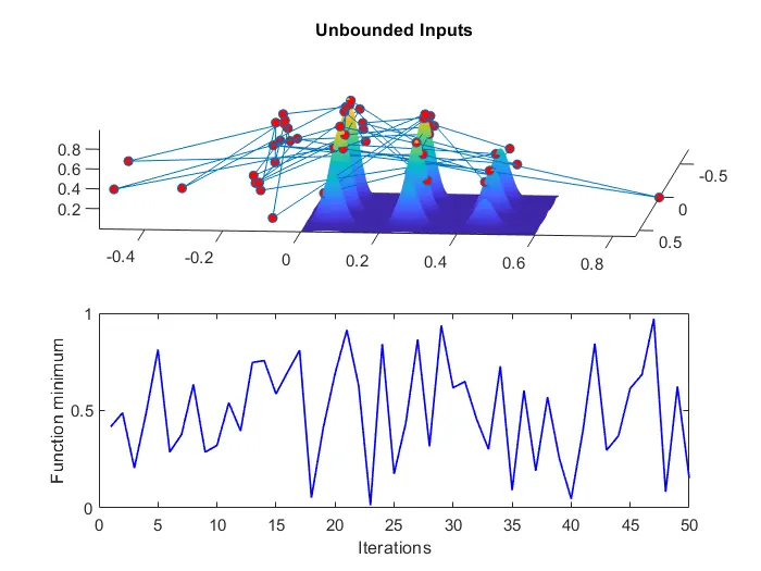
% Study 1 - Unbounded Condition
for i=1:num_cases
    [inputs,fopt(i)]=ga(@stalagmite_1,2);
    xopt(i)=inputs(1);
    yopt(i)=inputs(2);
end
studytime=toc

figure(1)
subplot(2,1,1) % To have multiple plots inside the same figure window
hold on
surfc(x,y,-f)
shading interp
plot3(xopt,yopt,-fopt,'marker','o','markersize',5,'markerfacecolor','r')
title('Unbounded Inputs')
subplot(2,1,2)
plot(-fopt,'color','b','linewidth',1)
xlabel('Iterations');
ylabel('Function minimum');

tic
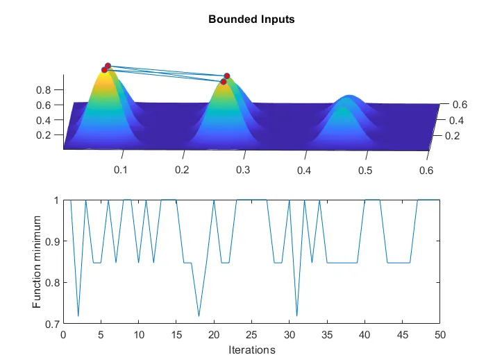
% Study 2 - Statistical behaviour - with upper and lower bounds
for i=1:num_cases
    [inputs,fopt(i)]=ga(@stalagmite_1,2,[],[],[],[],[0;0],[1;1]);
    xopt(i)=inputs(1);
    yopt(i)=inputs(2);
end
study2_time=toc;

figure(2)
subplot(2,1,1)
hold on
surfc(x,y,-f)
shading interp
plot3(xopt,yopt,-fopt,'marker','o','markersize',5,'markerfacecolor','r')
title('Bounded Inputs')
subplot(2,1,2)
plot(-fopt)
xlabel('Iterations');
ylabel('Function minimum');

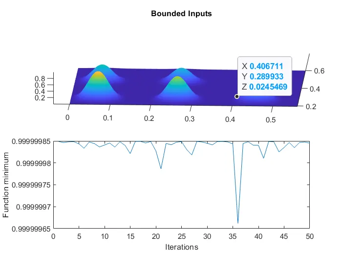
% Study 3 - Increasing GA Iterations
options=optimoptions('ga')
options=optimoptions(options,'PopulationSize',300);

tic
for i=1:num_cases
    [inputs,fopt(i)]=ga(@stalagmite_1,2,[],[],[],[],[0;0],[1;1],[],[],options);
    xopt(i)=inputs(1);
    yopt(i)=inputs(2);
end

study3_time=toc;

figure(3)
subplot(2,1,1)
hold on
surfc(x,y,-f)
shading interp
plot3(xopt,yopt,-fopt,'marker','o','markersize',5,'markerfacecolor','r')
title('Bounded Inputs')
subplot(2,1,2)
plot(-fopt)
xlabel('Iterations');
ylabel('Function minimum');

results-