Week 4.1 - Genetic Algorithm

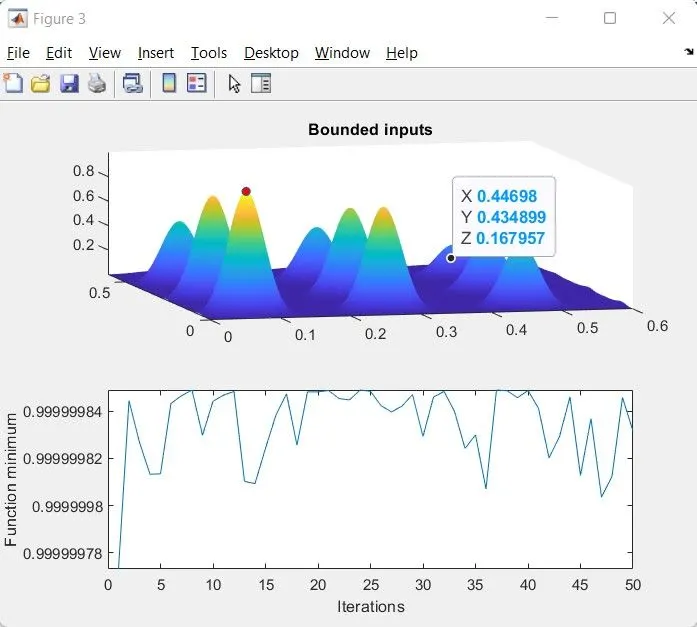
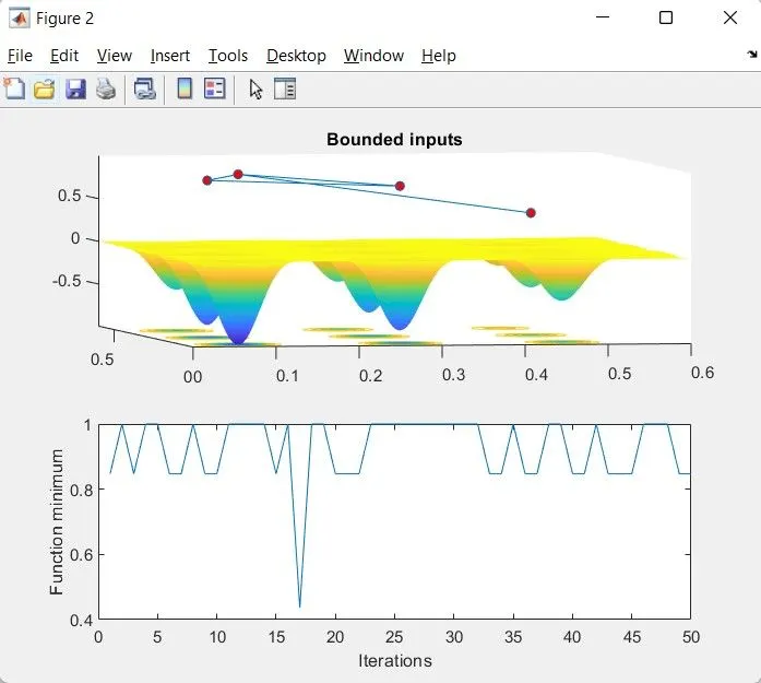
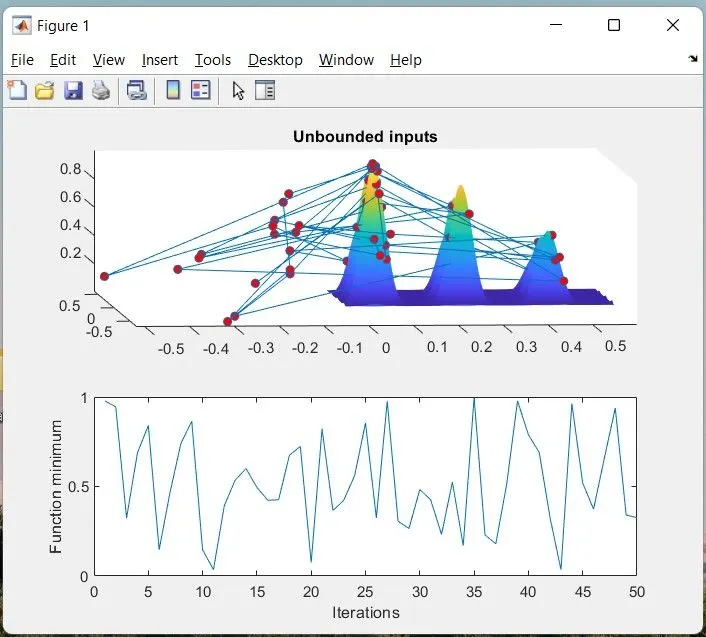
Genetic algorithm based upon the evolution theory that was proposed by the Jarvis Darvin, MATLAB provides the inbuild functions that actually help us the Genetic algorithm

Syntax

X = ga(fun, nvars)

Finds a local unconstrained minimum(x), to the objective function(fun) & Number of design variables of function(nvars)

codes:

clear all
close all
clc

x = linspace(0,0.6,150);
y = linspace(0,0.6,150);
num_cases = 50;
[xx,yy] = meshgrid(x,y);

for i=1:length(xx)
    for j=1:length(yy)
        input_vector(1)=xx(i,j);
        input_vector(2)=yy(i,j);
        f(i,j)=get_stalagmite(input_vector);
    end
end

tic
% Study 1 - satistical Behavior
for i = 1:num_cases
    [inputs, fopt(i)] = ga(@get_stalagmite, 2);
    xopt(i) = inputs(1);
    yopt(i) = inputs(2);
end
fopt = -fopt;
f = -f;
study1_time = toc

figure(1)
subplot(2,1,1)
hold on
surfc(x,y,f)
shading interp
plot3(xopt,yopt, fopt,'marker','o','markersize',5,'markerfacecolor','r')
title('Unbounded inputs')
subplot(2,1,2)
plot(fopt)
xlabel('Iterations')
ylabel('Function minimum')

tic
% Study 2 - Statistical behavior - with upper and lower bounds
for i = 1:num_cases
    [inputs, fopt(i)] = ga(@get_stalagmite,2,[],[],[],[],[0;0],[1;1]);
    xopt(i) = inputs(1);
    yopt(i) = inputs(2);
end
study2_time = toc
fopt = -fopt;
f = -f;
figure(2)
subplot(2,1,1)
hold on
surfc(x,y,f)
shading interp
plot3(xopt,yopt,fopt,'marker','o','markersize',5,'markerfacecolor','r')
title('Bounded inputs')
subplot(2,1,2)
plot(fopt)
xlabel('Iterations')
ylabel('Function minimum')

tic

%Study 3 increasing GA iteration
 options = optimoptions('ga');
 options = optimoptions (options, 'PopulationSize', 200);

for i = 1:num_cases
    [inputs, fopt(i)] = ga(@get_stalagmite,2,[],[],[],[],[0;0],[1;1],[],[],options);
    xopt(i) = inputs(1);
    yopt(i) = inputs(2);
end

fopt = -fopt;
f = -f;
study3_time = toc
figure(3)
subplot(2,1,1)
hold on
surfc(x,y,f)
shading interp
plot3(xopt,yopt,fopt,'marker','o','markersize',5,'markerfacecolor','r')
title('Bounded inputs')
subplot(2,1,2)
plot(fopt)
xlabel('Iterations')
ylabel('Function minimum')


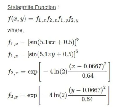
%Stalagmite

function f = get_stalagmite(input_vector)
x = input_vector(1);
y = input_vector(2);

f1x = (sin(((5.1*pi).*x)+0.5)).^6;
f1y = (sin(((5.1*pi).*y)+0.5)).^6;

f2x = exp((((x-0.0667).^2).*(-4*log(2)))./0.64);
f2y = exp((((y-0.0667).^2).*(-4*log(2)))./0.64);

f = -f1x*f1y*f2x*f2y;

end