Project 2 - Rankine cycle Simulator

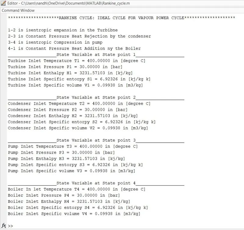
Output

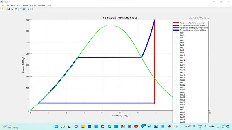
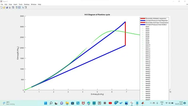
Plots

Code with explation

% Printing Introduction
fprintf('RANKINE CYCLE SIMULATOR\n')
fprintf('1-2 is isentropic empansion in the Turbibne\n')
fprintf('2-3 is Constant Pressure Heat Rejection by the condenser\n')
fprintf('3-4 is isentropic Compression in pump\n')
fprintf('4-1 is Constant Pressure Heat Addition ny the Boiler\n')

% User Inputs
P1 = input('Enter the pressure at the Turbine Inlet (in bar):');
T1 = input('Enter the Temperature at the Turbine Inlet (in Degree Celcius):');
P2 = input('Enter the Pressure at the Turbine Outlet(in bar):');

% State Point1
H1 = XSteam('h_pt',P1,T1); % Enthalpy
V1 = XSteam('v_pT',P1,T1); % Specific Volume
S1 = XSteam('s_pt',P1,T1); % Entropy
Hf1 = XSteam('hL_p',P1); % Enthalpy of Saturated liquid
Hg1 = XSteam('hV_p',P1); % Enthalpy of Saturated vapour
Ts1 = XSteam('Tsat_p',P1); % Saturation Temprature
Sf1 = XSteam('sL_p',P1); % Entropy of saturated liquid
Sg1 = XSteam('sV_p',P1); % Entropy of Saturated vapour

% State point 2
S2 = S1;
Sf2 = XSteam('sL_p',P2);
Sg2 = XSteam('sV_p',P2);
x = (S2-Sf2)/(Sg2-Sf2);
V2 = XSteam('v_ps',P2,S2);
Hf2 = XSteam('hL_p',P2);
Hg2 = XSteam('hV_p',P2);
H2 = Hf2 + x*(Hg2-Hf2);
T2 = XSteam('T_ph',P2,H2);
Ts2 = XSteam('Tsat_p',P2);

% State point 3
H3 = Hf2;
P3 = P2;
V3 = XSteam('vL_p',P3);
S3 = Sf2;
T3 = Ts2;


% State point 4
P4 = P1;
S4 = S3;
H4 = XSteam('h_ps',P4,S4);
T4 = XSteam('T_ps',P4,S4);
V4 = XSteam('v_ps',P4,S4);

t = linspace(280,374,500);

%Plot T-S Diagram
figure(1)
hold on
plot([S1 S2],[T1 T2],'Linewidth',5,'Color','r')
plot([S2 S3],[T2 T3],'Linewidth',5,'Color','b')
plot([S3 S4],[T3 T4],'Linewidth',5,'Color','r')
T = linspace(T4,T1,500);
for i = 1:length(T)
    s(i) = XSteam('s_pT',P1,T(i));
    h1(i) = XSteam('h_ps',P1,s(i));
    h2(i) = XSteam('h_ps',P2,s(i));
end
plot(s,T,'linewidth',5,'Color','b');
legend('Reversible Adiabatic expansion;','Constant Pressure Heat Rejection','Reversible Isentropic Compression','Constant Pressure Heat Addtion');

%Plot Ideal Ranking cycle in H -S Diagram
figure(2)
hold on
plot([S1 S2],[H1 H2],'LineWidth',5,'Color','r');
plot(s,h1,'LineWidth',5,'Color','b');
plot([S3 S4],[H3 H4],'LineWidth',5,'Color','r');
plot(s,h2,'LineWidth',5,'Color','b');
legend('Reversible Adiabatic expansion;','Constant Pressure Heat Rejection','Reversible Isentropic Compression','Constant Pressure Heat Addtion');
xlabel('Enthalpy[KJ/Kg]')
ylabel('Entropy[KJ/Kg_k]')
title('H-S Diagram of Rankine cycle')

%Plot T-S Diagram Saturation curve
t = linspace(0,374,500)
figure(1)
hold on
for i = 1 : length(t)
    plot(XSteam('sL_t',t(i)),t(i),'.','Color','g')
    plot(XSteam('sV_t',t(i)),t(i),'.','Color','g')
    hold on
end
figure(2)
hold on
for i = 1 : length(t)
    plot(XSteam('sL_t',t(i)),XSteam('hL_t',t(i)),'.','Color','g')
    plot(XSteam('sV_t',t(i)),XSteam('hV_t',t(i)),'.','Color','g')
    hold on
end

figure(1)
hold on
plot(S1,T1,'ko')
plot(S2,T2,'ko')
plot(S3,T3,'ko')
plot(S4,T4,'ko')
grid on
title('T-S Diagram of RANKINE CYCLE')
xlabel('Enthalpy[KJ/Kg]')
ylabel('Entropy[KJ/Kg_k]')


%Calculation
Wt = H1-H2
Wp = H4-H3
Qin = H1-H4
Qout = H2-H3
Wnet = Wt-Wp
Ntherm =(Wnet/Qin)*100
SSC = 3600/Wnet
BWR = Wp/Wt

%printing Results
fprintf('********************RANKINE CYCLE: IDEAL CYCLE FOR VAPOUR POWER CYCLE********************\n\n');
fprintf('1-2 is isentropic empansion in the Turbibne\n')
fprintf('2-3 is Constant Pressure Heat Rejection by the condenser\n')
fprintf('3-4 is isentropic Compression in pump\n')
fprintf('4-1 is Constant Pressure Heat Addition ny the Boiler\n')

fprintf('___________________State Variable at State point 1___________________\n');
fprintf('Turbine Inlet Temperature T1 = %.5f in [degree C]\n',T1);
fprintf('Turbine Inlet Pressure P1 = %.5f in [bar]\n',P1);
fprintf('Turbine Inlet Enthalpy H1 = %.5f in [kj/kg]\n',H1);
fprintf('Turbine Inlet Specific entorpy S1 = %.5f in [kj/kg k]\n',S1);
fprintf('Turbine Inlet Specific volume V1 = %.5f in [m3/kg]\n\n',V1);


fprintf('___________________State Variable at State point 2___________________\n');
fprintf('Condenser Inlet Temperature T2 = %.5f in [degree C]\n',T1);
fprintf('Condenser Inlet Pressure P2 = %.5f in [bar]\n',P1);
fprintf('Condenser Inlet Enthalpy H2 = %.5f in [kj/kg]\n',H1);
fprintf('Condenser Inlet Specific entorpy S2 = %.5f in [kj/kg k]\n',S1);
fprintf('Condenser Inlet Specific volume V2 = %.5f in [m3/kg]\n\n',V1);

fprintf('___________________State Variable at State point 3___________________\n');
fprintf('Pump Inlet Temperature T3 = %.5f in [degree C]\n',T1);
fprintf('Pump Inlet Pressure P3 = %.5f in [bar]\n',P1);
fprintf('Pump Inlet Enthalpy H3 = %.5f in [kj/kg]\n',H1);
fprintf('Pump Inlet Specific entorpy S3 = %.5f in [kj/kg k]\n',S1);
fprintf('Pump Inlet Specific volume V3 = %.5f in [m3/kg]\n\n',V1);

fprintf('___________________State Variable at State point 4___________________\n');
fprintf('Boiler In let Temperature T4 = %.5f in [degree C]\n',T1);
fprintf('Boiler Inlet Pressure P4 = %.5f in [bar]\n',P1);
fprintf('Boiler Inlet Enthalpy H4 = %.5f in [kj/kg]\n',H1);
fprintf('Boiler Inlet Specific entorpy S4 = %.5f in [kj/kg k]\n',S1);
fprintf('Boiler Inlet Specific volume V4 = %.5f in [m3/kg]\n\n',V1);