Week 4.1 - Genetic Algorithm

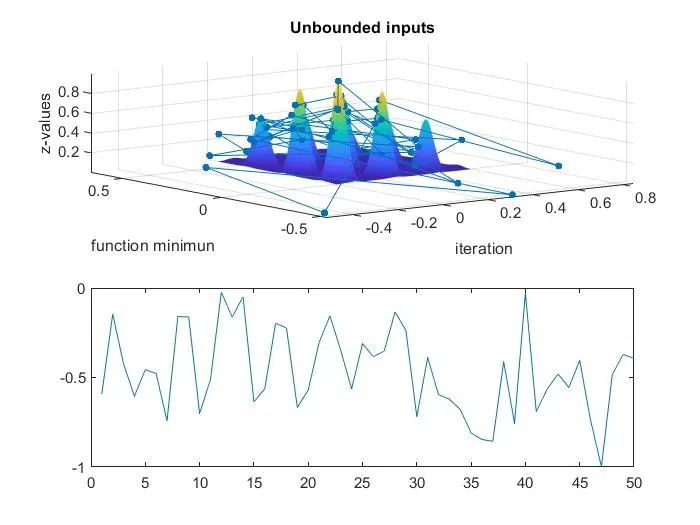
A genetic algorithm is a method for solving both constrained and unconstrained optimization problems based on a natural selection process that mimics biological evolution. The algorithm repeatedly modifies a population of individual solutions. use of stalagmite function is a mathematical model which helps us locate local maxima and minima. the optimization is used so that we can find global maxima without having prior knowledge of the function.

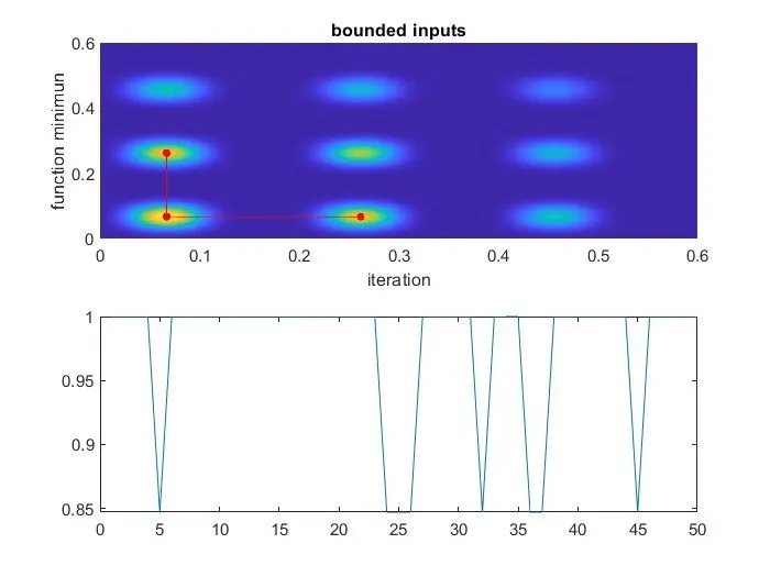
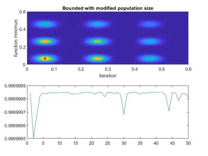
so to start first by creating 1-dimensional arrays and by that creating 2-dimensional arrays. using nested for loop and surfc command to visualize the function. then we perform the genetic algorithm (ga) command which is an in-built command. for this function to work we are passing 2 inputs: the function handler(the function we need to minimize) and how many variables are there in the function. by doing this we get 2 values negative and positive at which are function value is zero. then plot the graph, this is the first study. in the second study, we have given upper and lower bounds because of which the ga function gets a clearer idea or view, and the graph is much clearer but not correct, so in the third study we increased population six=ze with boundary conditions and got a correct global maxima.

%% genetic algorithm
clear all
close all
clc

%% PROVIDING THE SEARCH SPACE FOR THE FUNCTION
x = linspace(0,0.6,150);
y = linspace(0,0.6,150);
 
[xx,yy] = meshgrid (x,y);
%% CREATING THE SURFACE PLOT OF STALAGEMITE FUNCTION
for i = 1: length(x)
    for j = 1:length(y)
        input(1) = xx(i,j);
        input(2) = yy(i,j);
        f(i,j) = stalagmite(input);  %values of function in given search space
    end
end

%% study 1 unbound condition
for k = 1:50  %number of cases

    [input,fopt(k)] = ga(@stalagmite,2);
    xopt(k) = input(1);
    yopt(k) = input(2);

end
figure(1)
subplot(2,1,1)
surfc(x,y,-f)  %generating the surface
xlabel('iteration')
ylabel('function minimun')
zlabel('z-values')
shading interp   %To remove the lines produced by the mesh grid
hold on
%plotting
plot3(xopt,yopt,-fopt,'marker','.','markersize',10);
title('Unbounded inputs')
subplot(2,1,2)
plot(fopt)

tic

%% STATISTICAL BEHAVIOUR (BOUNDED)
for i = 1:50     %number of cases
    [input, fopt(i)] = ga(@stalagmite,2,[],[],[],[],[0;0],[0.4;0.4]);   %calculating the optimized value of the function
      xopt(i) = input(1);
      yopt(i) = input(2);
end
study2_time = toc   %displaying the time taken to evaluate

figure(2)
subplot(2,1,1)
hold on
surfc(x,y,-f)    %generating the surface
shading interp    %To remove the lines produced by the mesh grid
%plotting
plot3(xopt, yopt, -fopt,'marker','.','MarkerSize',10,'Color','r')
title('bounded inputs')
xlabel('iteration')
ylabel('function minimun')
zlabel('z-values')
subplot(2,1,2)
plot(-fopt)

%study 3- increasing GA iteration
%% MODIFYING THE NUMBER OF POPULATION
options = optimoptions('ga')
options = optimoptions(options,'PopulationSize',200)

tic
for i = 1:50   %number of cases
    [input, fopt(i)] = ga(@stalagmite,2,[],[],[],[],[0;0],[0.4;0.4],[],[],options);
      xopt(i) = input(1);
      yopt(i) = input(2);
end
study3_time = toc   %displaying the time taken to evaluate

figure(3)
subplot(2,1,1)
hold on
surfc(x,y,-f)    %generating the surface
shading interp    %To remove the lines produced by the mesh grid
%plotting
plot3(xopt, yopt, -fopt,'marker','.','MarkerSize',10,'Color','r')
title('Bounded with modified population size')
xlabel('iteration')
ylabel('function minimun')
zlabel('z-values')
subplot(2,1,2)
plot(-fopt)