Week 3 - Taylor table method and Matlab code
Challenge 5 week 3
(submitted by Kurias.M.George)
OBJECTIVE
Derive the following 4th order approximations of the second-order derivative.
1. Central difference
2. Skewed right-sided difference
3. Skewed left-sided difference
After deriving these schemes, prove that your skewed schemes are fourth-order accurate i.e the thumb rule given in HINT (ii).
Once you have done this, write a program in Matlab to evaluate the second-order derivative of the analytical function exp(x)*cos(x) and compare it with the 3 numerical approximations that you have derived.
Provide a plot that compares the absolute error between the above-mentioned schemes
In your own words, describe why a skewed scheme is useful? What can a skewed scheme do that a CD scheme cannot?
METHODOLOGY
Initially u we have, f(x) = exp(x)*cos(x)
we give x= pi/3;
we assign f(x)=y
we can compute the analytical derivative of y as y_1 = y_1= -exp(x)*(cos(x)-sin(x))
we find the value derivative y_1 analytically at x=pi/3
dx = linspace(pi/30,pi/300,20)
then we compute the the Left , Right and skewed elements
Then we go for the Numerical dericvatives
then we plot the the errors on the bar graph
CALCULATIONS
skewed forward differencing
`(Delta)*( x^2)*(d^2 u)/(dx^2 )= a *f(i) + b*f(i+1)+ c*f(i+2)+d*f(i+3)+e*f(i+4)+f*f(i+5)`)
p+q = 2+4 =6
| `f(i)` | Deltax *f(i) | Deltax^2 * f(i) | Deltax^3 *f(i) | Deltax^4*f(i) | Deltax^5 *f(i) | |
| a *f(i) | a | 0 | 0 | 0 | 0 | 0 |
| b *f(i+1) | b | b | b/2 | b/6 | b/24 | b/120 |
| c *f(i+2) | c | 2c | 4c/2 | 8c/6 | 16c/24 | 32c/120 |
| d *f(i+3) | d | 3d | 9d/2 | 27d/6 | 81d/24 | 243d/120 |
| e *f(i+4) | e | 4e | 16e/2 | 64e/6 | 256e/24 | 1024e/120 |
| g *f(i+5) | g | 5g | 25g/2 | 125g/6 | 625g/24 | 3125g/120 |
a+b+c+d+e+g= 0 ...........(1)
b+2c+3d+4e+5g=0...............(2)
b/2+4c/2+9d/2+16e/2+25g/2=1...........(3)
b/6+8c/6+27d/6+64e/6+125g/6=0................(4)
b/24+16c/24+81d/24+256e/24+625g/24=0...............(5)
b/120+32c/120+243d/120+1024e/120+3125g/120=0...........(6)
onsolving 1,2,3,4,5 we get the values for a,b,c,d,e and g
a=3.7500
b=-12.8333
c=17.8333
d=-13.0000
e=5.0833
g=-0.8333
skewed backward differencing(left)
`(Deltax^2)*(d^2 u)/dx^2 = a *f(i-5) + b*f(i-4)+ c*f(i-3)+d*f(i-2)+e*f(i-1)+g*f(i)`
| `f(i)` | `Deltax *f(i)` | `Deltax^2 * f(i)` | `Deltax^3 *f(i)` | `Deltax^4*f(i) | `Deltax^5 *f(i)` | |
| a *f(i-5) | a | -5a | 25a/2 | -125a/6 | 625a/24 | -3125a/120 |
| b *f(i-4) | b | -4b | 16b/2 | -64b/6 | 256b/24 | -1024b/120 |
| c *f(i-3) | c | -3c | 9c/2 | -27c/6 | 81c/24 | -243c/120 |
| d *f(i-2) | d | -2d | 4d/2 | -8d/6 | 16d/24 | -32d/120 |
| e *f(i-1) | e | -e | e/2 | -e/6 | e/24 | -e/120 |
| g *f(i) | g | 0 | 0 | 0 | 0 | 0 |
a+b+c+d+e+g= 0 ...........(1)
-(e+2d+3c+4b+5a)=0...............(2)
e/2+4d/2+9c/2+16b/2+25a/2=1...........(3)
-(e/6+8d/6+27c/6+64b/6+125a/6)=0............(4)
e/24+16d/24+81c/24+256b/24+625a/24=0...............(5)
-(e/120+32d/120+243c/120+1024b/120+3125a/120)=0...........(6)
onsolving 1,2,3,4,5 we get the values for a,b,c,d,e and g
a=-0.8333
b=5.0833
c=-13.0000
d=17.8333
e=-12.8333
g=3.7500
central differencing
`(Deltax^2)*(d^2 u)/dx^2 = a *f(i-2) + b*f(i-1)+ c*f(i)+d*f(i+1)+e*f(i+2)`
`P+Q-1`= 2+4-1 =5
| `f(i)` | `Deltax *f(i)` | `Deltax^2 * f(i)` | `Deltax^3 *f(i)` | `Deltax^4*f(i)` | `Deltax^5 *f(i)` | |
| a *f(i-2) | a | -2a | 4a/2 | -8a/6 | 16a/24 | -32a/120 |
| b *f(i-1) | b | -b | b/2 | -b/6 | b/24 | -b/120 |
| c *f(i) | c | 0 | 0 | 0 | 0 | 0 |
| d *f(i+1) | d | d | d/2 | d/6 | d/24 | d/120 |
| e *f(i+2) | e | 2e | 4e/2 | 8e/6 | 16e/24 | 32e/120 |
a+b+c+d+e= 0 ...........(1)
-2a-b+d+2e=0...............(2)
4a/2+b/2+d/2+4e/2=1...........(3)
-8a/6+-b/6+d/6+8e/6=0................(4)
16a/24+b/24+d/24+16e/24=0...........(5)
onsolving 1,2,3,4,5 we get the values for a,b,c,d,e and g
a=-0.0833
b=1.3333
c=-2.5000
d=1.3333
e=-0.0833
CODING
descritization function
clear all
close all
clc
x=pi/3;
dx = linspace(pi/30,pi/300,20);
% Function : y=exp(x)*cos(x);
Analytical_derivative_1st = -exp(x)*(cos(x)-sin(x)) ;
Analytical_derivative_2nd = -2*exp(x)*sin(x);
%Taylor table for Left skewed scheme
A =[1 1 1 1 1 1;-5 -4 -3 -2 -1 0;25/2 16/2 9/2 4/2 1/2 0;-125/6 -64/6 -27/6 -8/6 -1/6 0;625/24 256/24 81/24 16/24 1/24 0;-3125/120 -1024/120 -243/120 -32/120 -1/120 0] ;
B = [0;0;1;0;0;0];
%Taylor table for Right skewed scheme
C =[1 1 1 1 1 1;0 1 2 3 4 5;0 1/2 4/2 9/2 16/2 25/2;0 1/6 8/6 27/6 64/6 125/6;0 1/24 16/24 81/24 256/24 625/24;0 1/120 32/120 243/120 1024/120 3125/120];
D = [0;0;1;0;0;0];
%Taylor table for Central scheme
E = [1 1 1 1 1;-2 -1 0 1 2;4/2 1/2 0 1/2 4/2;-8/6 -1/6 0 1/6 8/6;16/24 1/24 0 1/24 16/24];
F = [0;0;1;0;0];

X =  Left_Skewed(A,B); % N = P(Order of derivative) + Q(Order of approx.)
Y =  Right_Skewed(C,D); % N = P(Order of derivative) + Q(Order of approx.)
Z = Central(E,F); % N = P(Order of derivative) + Q(Order of approx.) - 1

for i =1:length(dx)

 [LSS RSS CS] = Numerical_derivative(x,dx(i),X,Y,Z);

 error_left(i) = abs(LSS - Analytical_derivative_2nd);
 error_right(i) = abs(RSS - Analytical_derivative_2nd);
 error_central(i) = abs(CS - Analytical_derivative_2nd);

end


% loglog(dx,error_left(i),'r')
% hold on
% loglog(dx,error_right(i),'b')
% loglog(dx,error_central(i),'g')

plot(dx,error_central(i),'o')
hold on
plot(dx,error_right(i),'x')
plot(dx,error_left(i),'*')
xlabel('errors')
ylabel('dx')
function
function y = fofx(x)
y  = exp(x)*cos(x);
end
Left skewed
function out = Left_Skewed(g,h)
out = inv(g)*h;
end
right skewed
function out = Right_Skewed(g,h)
out = inv(g)*h;
end
central skewed
function out = Central(g,h)
out = inv(g)*h;
end
Numerical dericative
function [left right central] = Numerical_derivative(x,dx,X,Y,Z)

left = ((X(1)*fofx(x-(5*dx)))- ((X(2)*fofx(x-(4*dx)))+(X(3)*fofx(x-(3*dx)))-(X(4)*fofx(x-(2*dx)))+(X(5)*fofx(x-(1*dx)))-(X(6)*fofx(x))))/(dx^2);

right = ((Y(1)*fofx(x))+(Y(2)*fofx(x+dx))+(Y(3)*fofx(x+(2*dx)))+(Y(4)*fofx(x+(3*dx)))+(Y(5)*fofx(x+(4*dx)))+(Y(6)*fofx(x+(5*dx))))/(dx^2);

central = ((Z(1)*fofx(x-(2*dx)))+(Z(2)*fofx(x-dx))+(Z(3)*fofx(x))+(Z(4)*fofx(x+dx))+(Z(5)*fofx(x+(2*dx))))/dx^2;

end
RESULTS
The analytical derivative is initially found out using the mathematical equations.
The numerical dericvative is found out using the different methods, using the skewed left, right and central. the values are promising with the right patterns being shown at the results which can be observed easily.
the graph of errors is obrained as
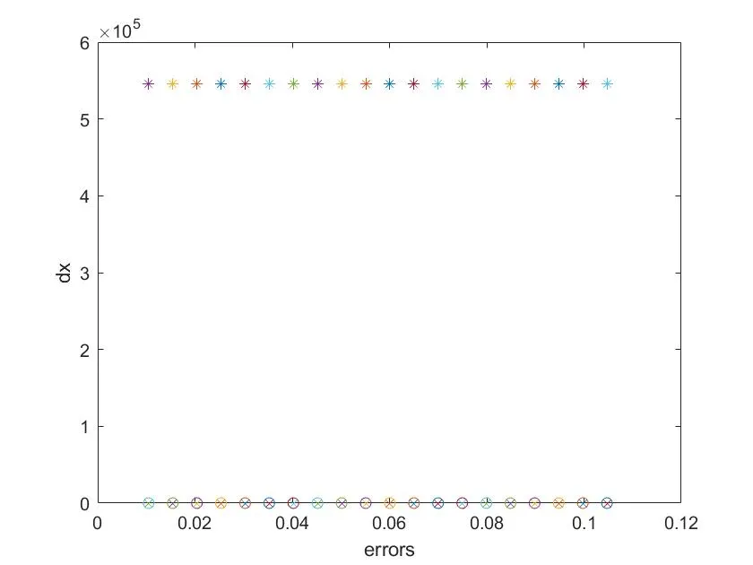
The skewed method is useful for finding the numerical dericvatives more accrately. We can see that the central and right error are similar and also thers is some hype in the value of the error to dx graph in the left skew method which can be due to the dissimilarities and round of errors.
LEARNING OUTCOMES
learned to compare analytical and numerical derivatives of functions
CONCLUSION
for the given function, the analytical derivative has been found and then comapred withnumerical derivatives. we can see that the left skewed error is showing some abnormalities. ie, showing somw higher values of errors and this can be due to the round off errors.