Taylor table method and MATLAB code

Aim:

To write program using MATLAB to derive 4^th order approximation of the second-order derivative. And to evaluate the second-order derivative of the given analytical function.

Introduction:

The FDM is for replacing the partial derivative appearing in governing equations of fluid dynamics, with algebraic difference quotients yielding a system of algebraic equations which can be solved for the flow field variables at specific, discrete grid points in the equation.

Central difference scheme:

TERMS	f(i)	Δ(x)*f’(i)	Δ(x)^2*f’’(i)	Δ(x)^3*f’’’(i)	Δ(x)^4*f’’’’(i)	Δ(x)^5*f’’’’’(i)
f(i-2)	a	-2a	4a/2	-8a/6	-16a/24	-32a/120
f(i-1)	b	-b	b/2	-b/6	b/24	-b/120
f(i)	c	0	0	0	0	0
f(i+1)	d	d	d/2	d/6	d/24	d/120
f(i+2)	e	2e	4e/2	8e/6	16e/24	32e/120
summation	0	0	1	0	0	0

Skewed right sided scheme:

TERMS	f(i)	Δ(x)*f’(i)	Δ(x)^2*f’’(i)	Δ(x)^3*f’’’(i)	Δ(x)^4*f’’’’(i)	Δ(x)^5*f’’’’’(i)
f(i)	a	0	0	0	0	0
f(i+1)	b	b	b/2	b/6	b/24	b/120
f(i+2)	c	2c	4c/2	8c/6	0	32c/120
f(i+3)	d	3d	9d/2	27d/6	d/24	245d/120
f(i+4)	e	4e	16e/2	64e/6	16e/24	1024e/120
summation	0	0	1	0	0	0

Skewed left sided scheme:

TERMS	f(i)	Δ(x)*f’(i)	Δ(x)^2*f’’(i)	Δ(x)^3*f’’’(i)	Δ(x)^4*f’’’’(i)	Δ(x)^5*f’’’’’(i)
f(i)	a	0	0	0	0	0
f(i-1)	b	-b	b/2	-b/6	b/24	-b/120
f(i-2)	c	-2c	4c/2	-8c/6	0	-32c/120
f(i-3)	d	-3d	9d/2	-27d/6	d/24	-245d/120
f(i-4)	e	-4e	16e/2	-64e/6	16e/24	-1024e/120
summation	0	0	1	0	0	0

Formula for finding number of terms:

N = [A+O-1]

N = [4+2-1] = 5

N = number of terms

A = order of approximation

O = order of derivative

Program for derivation of the formula for second-order derivative with fourth-order approximation

%program to solve taylor table

clear all
close all
clc

%central difference taylor table
[A] = [1 1 1 1 1;
       -2 -1 0 1 2;
       2 1/2 0 1/2 2;
       -8/6 -1/6 0 1/6 8/6;
       16/24 1/24 0 1/24 16/24];
[B] = [0;0;1;0;0];
[X] = linsolve(A,B) %solving for co efficient of matrix

%skewed right sided difference
[C] = [1 1 1 1 1;
       0 1 2 3 4;
       0 1/2 2 9/2 8;
       0 1/6 4/3 9/2 32/3;
       0 1/24 2/3 27/8 32/3];
[D] = [0;0;1;0;0];
[Y] =linsolve(C,D)

%skewed left sided difference
[E] = [1 1 1 1 1;
       0 -1 -2 -3 -4;
       0 1/2 2 9/2 8;
       0 -1/6 -4/3 -9/2 -32/3;
       0 1/24 2/3 27/8 32/3];
[F] = [0;0;1;0;0];
[Z] = linsolve(E,F)

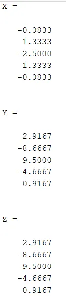
output for above code

Forward and backward difference scheme:

clear all
close all
clc

%initial parameters for the given system
x = pi/3;
dx = linspace(pi/4, pi/400,100);

%analytical fuction = exp^(x)*cos(x)

analytical_derivative = -2*exp(x)*sin(x);

for i = 1:length(dx)
    %taylor series function at various node points
    a(i) = (exp(x-(5*dx(i)))*cos(x-(5*dx(i))));
    b(i) = (exp(x-(4*dx(i)))*cos(x-(4*dx(i))));
    c(i) = (exp(x-(3*dx(i)))*cos(x-(3*dx(i))));
    d(i) = (exp(x-(2*dx(i)))*cos(x-(2*dx(i))));
    e(i) = (exp(x-dx(i))*cos(x-dx(i)));
    f(i) = (exp(x)*cos(x));
    g(i) = (exp(x+dx(i))*cos(x+dx(i)));
    h(i) = (exp(x+(2*dx(i)))*cos(x+(2*dx(i))));
    j(i) = (exp(x+(3*dx(i)))*cos(x+(3*dx(i))));
    k(i) = (exp(x+(4*dx(i)))*cos(x+(4*dx(i))));
    l(i) = (exp(x+(5*dx(i)))*cos(x+(5*dx(i))));
    
    %expression formulas for varioius taylor series functions
    %forward difference scheme
    forward_difference(i) = (g(i)-f(i))/(dx(i));
    
    %backward difference scheme
    backward_difference(i) = (f(i)-e(i))/(dx(i));
    
    %central difference scheme
    central_difference(i) = (-1*(d(i))+16*(e(i))-30*(f(i))+16*(g(i))-1*(h(i)))/(12*dx(i)^2);
    
    %skewed left sided difference
    skew_left(i) = (45*(f(i))-154*(e(i))+214*(d(i))-156*(c(i))+61*(b(i))-10*(a(i)))/(12*(dx(i)^2));
    
    %skewed right sided difference
    skew_right(i) = (45*(f(i))-154*(g(i))+214*(h(i))-156*(j(i))+61*(k(i))-10*(l(i)))/(12*(dx(i)^2));
    
    %error
    error_forward(i) = abs(forward_difference(i) - analytical_derivative);
    error_backward(i) = abs(backward_difference(i) -analytical_derivative);
    error_central(i) = abs(central_difference(i) -analytical_derivative);
    error_left(i) = abs(skew_left(i) - analytical_derivative);
    error_right(i) = abs(skew_right(i) - analytical_derivative);
end

figure(1)
subplot(1,2,1)
loglog(dx,error_forward,'linewidth',1,'marker','hexagram')
xlabel('dx')
ylabel('Absolute Error')
title('Absolute Error in Difference scheme v/s dx')
grid on
hold on
loglog(dx,error_backward,'linewidth',1,'marker','pentagram')
xlabel('dx')
ylabel('Absolute Error')
legend('Forward difference scheme','Backward difference scheme')
subplot(1,2,2)
loglog(dx,error_right,'linewidth',1,'marker','hexagram')
xlabel('dx')
ylabel('Absolute Error')
title('Absolute Error in various finite difference schemes')
grid on
hold on
loglog(dx,error_left,'linewidth',1,'marker','pentagram')
xlabel('dx')
ylabel('Absolute Error')
grid on 
hold on
loglog(dx,error_central,'linewidth',1,'marker','d')
xlabel('dx')
ylabel('Absolute error')
grid on
legend('skewed right sided difference','skewed left sided difference','central difference scheme')

%to find exact slope of the curve
L_1 = log10(dx);
L_2 = log10(error_forward);
L_3 = log10(error_backward);
L_4 = log10(error_right);
L_5 = log10(error_left);
L_6 = log10(error_central);
%g_1 = gradient(L_2,L_1);
%g_2 = gradient(L_3,L_1);
g_3 = gradient(L_4,L_1);
g_4 = gradient(L_5,L_1);
g_5 = gradient(L_6,L_1);

figure(2)
plot(g_3,'linewidth',1,'marker','pentagram')
hold on
plot(g_4,'linewidth',1,'marker','hexagram')
plot(g_5,'linewidth',1,'marker','d')
legend('skewed right sided difference','skewed left sided difference','central difference scheme')
title('slope of the curve')

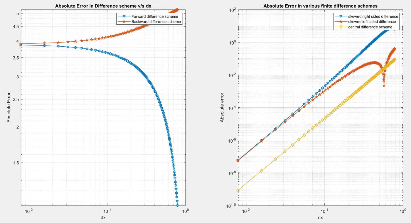
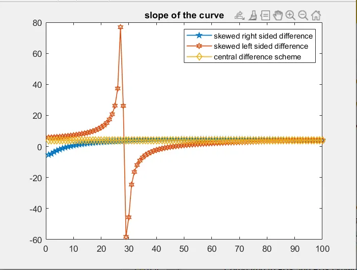
Plots:

in your own words, describe why a skewed scheme is useful? What can a skewed scheme do that a CD scheme cannot do?

The skewed scheme works well when no of points available on one side of the grid. Indeed, for calculating corner node with higher approximations we need skewed at this point for this type no longer central scheme useful.

Forward difference and backward difference schemes require information on the right and left neighboring points respectively. In FDS and BDS it solves the equation with 1^st order approximation with 1^st order derivative and the central differencing scheme solve the equation with 2^nd order approximation with 1^st order derivative both are using same two-point information but CDS provides more accurate results.

Compared to FDS and BDS skewed scheme provides a more accurate result because of getting more available information from many points. It can be used for solving when points available on one side. But the central difference can we use for solving two sides because of its symmetric nature. Higher the order lower the error for the same grid sizes.

The graph and output values obtained above for central difference, forward difference scheme, backward difference scheme, skewed right scheme, skewed left scheme we can clearly understand that central difference scheme contains less error compared to all other schemes.

Result:

The program is written using MATLAB to derive 4^th order approximation of the second-order derivative. And to evaluate the second-order derivative of the given analytical function. The plots are as given above.