Program for Air standard cycle- OTTO CYCLE using MATLAB

Aim:

To write a program using MATLAB to plot PV diagram for air standard cycle – otto cycle.

Introduction:

Otto- cycle :

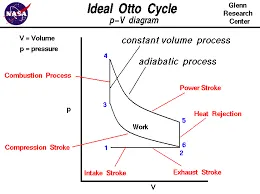
Otto cycle is an air standard cycle which approximates the processes in petrol and diesel engines. It is based on constant volume heat addition and constant volume heat rejection processes and isentropic compression and expansion. The below diagram shows the otto cycle,

Thermal efficiency:

It is defined as the ratio of work done to heat gain. The formula for thermal efficiency is given below.

And the formula for thermal efficiency for otto cycle is as given below:

Derived formula for thermal efficiency for otto cycle.

Where,

CR = compression ratio

Program for air standard cycle using MATLAB is given below:

% program for air standard cycle - otto cycle

%engine geometric parameters

bore =0.1 ;

stroke = 0.1;

con_rod = 0.15;

cr = 8;

%inputs

gamma = 1.4;

%calculating for swept volume and clearance volume

v_swept = (pi/4)*bore^2*stroke ;

v_clearance = v_swept/(cr-1);

%state variables at state point 1

t1 = 300 ;

p1 = 10000;

v1 = v_swept + v_clearance;

%State variables at state point 2

%p2v2^gamma = p1v1^gamma || p2 = p1*cr^gamma

p2 = p1*cr^gamma ;

%p1*v1*t1 = p2*v2*t2 || t2 = (p2*v2*t1)/(p1*v1)

v2 = v_clearance ;

t2 = (p2*v2*t1)/(p1*v1);

%isentropic compression

constant_c = p1*v1^gamma;

v_compression = engine_kinematics(bore, stroke, con_rod, cr, 180, 0);

p_compression = constant_c./v_compression.^gamma;

%state variables at state point 3

t3 = 1200;

v3 = v2;

%(p3*v3)/t3 = (p2*v2)/t2 || p3 = (p2*v2*t3)/(v3*t2)

p3 = (p2*t3)/(t2) ;

%isentropi expansion

constant_c = p3*v3^gamma;

v_expansion = engine_kinematics(bore, stroke, con_rod, cr, 0,180);

p_expansion = constant_c./v_expansion.^gamma;

%state variables at state point 4

v4 = v1;

%p4*v4^gamma = p3*v3^gamma || p4 = p3*(v3/v4)^gamma || p4 = p3*(1/cr)^gamma

p4 = p3*(1/cr)^gamma;

%thermal efficiency for otto cycle

thermal_efficiency = 1-(1/(cr^(gamma-1)))

%plot for state points

figure(1)

hold on

plot(v1,p1,'*','color','r');

plot(v2,p2,'*','color','r');

plot(v3,p3,'*','color','r');

plot(v4,p4,'*','color','r');

plot(v_compression, p_compression,'m');

plot([v2 v3],[p2 p3],'color','g');

plot(v_expansion, p_expansion,'b');

plot([v4 v1],[p4 p1],'color','g');

xlabel('Volume');

ylabel('Pressure');

title('OTTO CYCLE PLOT');

grid on

function for engine kinematics is as below:

function [V] = engine_kinemaitcs(bore, stroke, con_rod, cr, start_crank, end_crank)

a = stroke/2;

R = con_rod/a;

v_s = (pi/4)*bore^2*stroke ;

v_c = v_s/(cr-1);

theta = linspace(start_crank, end_crank, 100);

term1 = 0.5*(cr-1);

term2 = R+1-cosd(theta);

term3 = (R^2-sind(theta).^2).^0.5;

V = (1+ term1 *(term2 - term3)).*v_c;

end

explanation for program:

The program is initiated with the known engine parameters. Those are bore, stroke, connecting rod length, compression ratio, gamma. Here the values engine parameters are assumed as follows,

Bore = 0.1 meters;

Stroke = 0.1 meters;

Connecting rod length = 0.15 meters;

Compression ratio = 8 ;

Gamma = 1.4;

The state variables are calculated using the below relations,

i.e P1*V1^gamma = P2*V2^gamma and (P1*V1)/T1 = (P2*V2)/T2

swept volume and clearance volume of the engine is calculated as follows

v_swept = (pi/4)*bore^2*stroke ;

v_clearance = v_swept/(cr-1);

function for engine kinematics:

a function is created as engine_kinematics and inputs are bore, stroke, con_rod, cr, start_crank, end_crank. The formula used here is as follows:

V = 1 + 0.5*(CR-1)[R+1-Cos(theta)-(R^2-(Sin(theta))^2)^0.5]

For simplification, I have taken 3 terms as follows:

Term1 = 0.5*(cr-1);

Term2 = R+1-cosd(theta);

Term3 = (R^2-sind(theta).^2).^0.5;

screenshot of the P-V diagram for otto cycle using MATLAB is below,

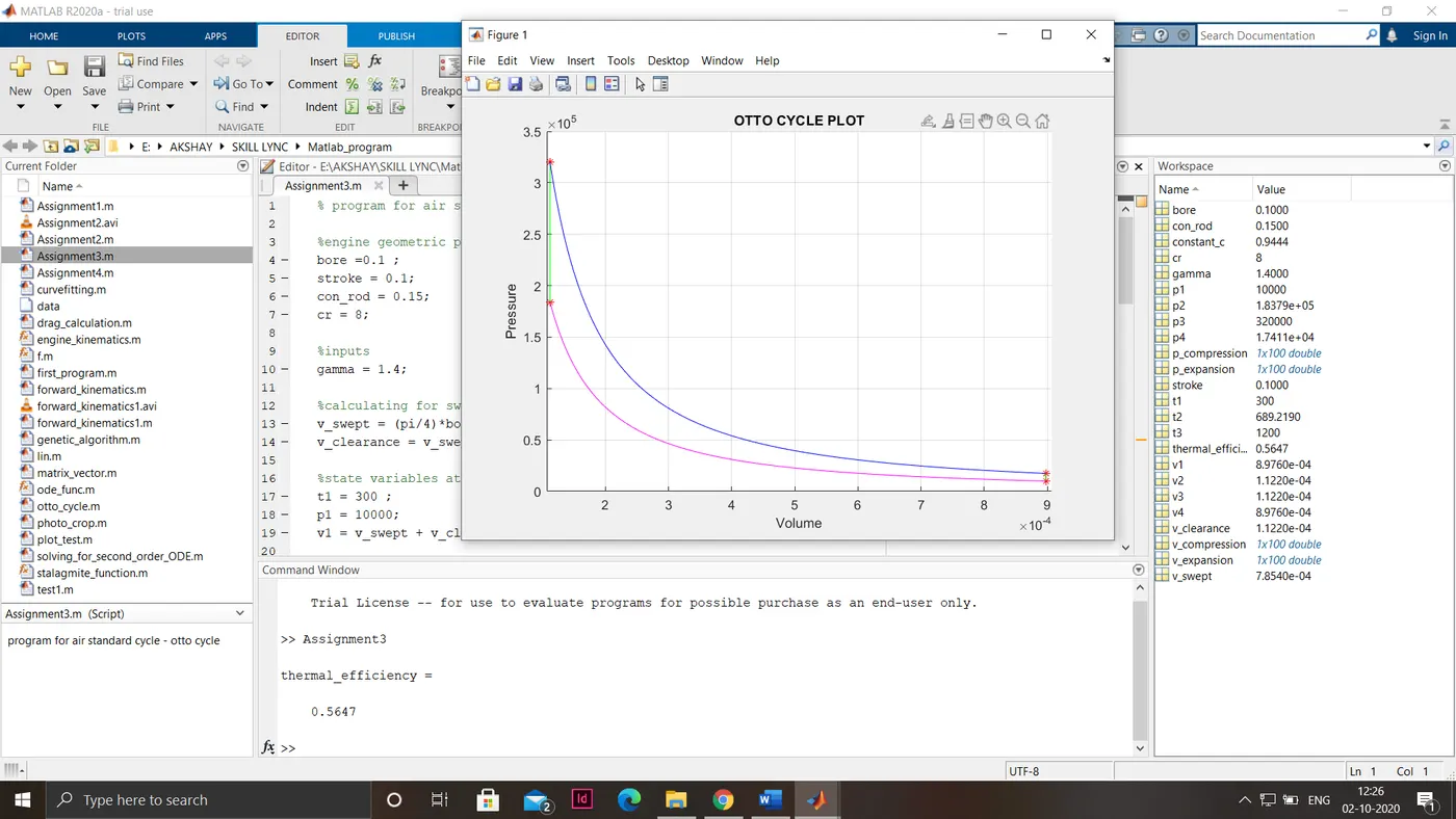
Figure shows the otto cycle and output thermal efficiency in the command window.

Result:

P-V diagram for the otto cycle is plotted and thermal efficiency is displayed as output.