Program to simulate the motion of pendulum using MATLAB

Aim:

To write a program to solve the second order ODE and simulate the motion of pendulum using MATLAB.

Introduction:

A differential equation is an equation for a function that relates the values of the function to the values of its derivatives. An ordinary differential equation (ode) is a differential equation for a function of a single variable. where as the partial differential equation(pde) is a differential equation for function of several variables.

The given differential equation is as follows:

Where,

g = gravity in m/s2,

L = length of the pendulum in m,

m = mass of the ball in kg,

b=damping coefficient

and the values for above mentioned variables are given below:

L=1 metre,

m=1 kg,

b=0.05.

g=9.81 m/s2.

Using above given information and equation the program for solving ode and simulation for motion of the pendulum is as below.

Program for solving second order ODE and simulation of motion of pendulum.

%program to solve second order ODE and to simulate the motion of the pendulum
 
clear all
close all
clc
 
b = 0.05;
g = 9.81;
l = 1;
m = 1;
 
%initial conditions
 
theta_0 = [0;3];
%time span
t_span = linspace(0,20,100);
 
%solvefor ODE
[t, result] = ode45(@(t, theta) ode_function(t,theta,b,g,l,m), t_span, theta_0);
 
plot(t, result(:,1));
hold on
plot(t, result(:,2));
ylabel('plot');
xlabel('time');
 
%program to simulate the motion of pendulum
fig = 1;
for i = 1:length(t);
    %initial positon of the pendulum
    xo = 0;
    yo = 0;
    
    %final positon 
    
    x1 = l*sin(result(i,1));
    y1 = -l*cos(result(i,1));
    
    %plotting 
    figure(2)
    %base line
    plot([-0.5 0.5],[0 0], 'linewidth', 3, 'color','g');
    hold on
    % pendulum length
    plot([xo x1],[yo y1], 'linewidth', 3,'color', 'k');
    %pendulum ball
    plot(xo, yo, 'o','markers', 5, 'markerfacecolor', 'r');
    plot(x1, y1, 'o','markers', 20, 'markerfacecolor', 'r')
    axis([-1 1 -1.5 0.5])
    grid on
    hold off
    pause(0.1);
    M(fig) = getframe(gcf);
    fig = fig + 1;
end
movie(M)
videofile = VideoWriter('motion_of_pendulum.avi','Uncompressed AVI' );
open(videofile)
writeVideo(videofile,M)
close(videofile)

Explanation for program:

The program is written using MATLAB. With reference to the given values and information the program is written as shown above.

Ode45 function is the inbuilt ordinary differential equation function with the syntax as [t,y] = ode45(odefun,tspan,y0).here in our program the odefun is defined as ode_function(t,theta,b,g,l,m).

where, t, theta , b, g, l,m are inputs to the function. Ode_function is as below:

%ode function
function [dtheta_dt] = ode_function(t,theta,b,g,l,m);

    theta1 = theta(1);
    theta2 = theta(2);
    dtheta1_dt = theta2;
    dtheta2_dt = -(b/m)*theta2 - (g/l)*sin(theta1);
    
    dtheta_dt = [dtheta1_dt; dtheta2_dt];
end

The pendulum is drawn using plot command providing the co ordinates of the line. The bob or mass is drawn using marker command. The animation is done giving the pause of 0.1 second and animation is recorded.

The link of the animation is attached here: https://drive.google.com/file/d/1VB91mRnIsnbVvvrK_r5lMbuIEpqm2Psa/view?usp=sharing

Plot:

The plots as result of solving second order ODE is as shown below:

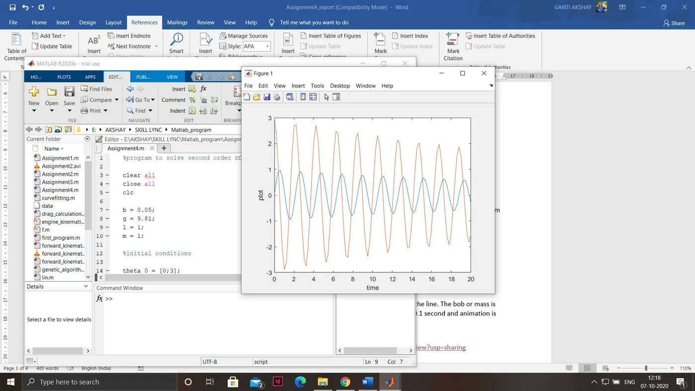
figure shows the plot vs time graph.

Result:

The second order ode is solved using MATLAB and the animation for the motion of pendulum is done and attached here.