Week 3 - Solving second order ODEs

Aim :

write a program that solves the following ODE. This ODE represents the equation of motion of a simple pendulum with damping

Governing equation :

equation of motion of a simple pendulum with damping

`(d^2theta)/dt^2 +(b/m) ((d theta)/(dt))+ (g/l)sintheta`

where ,

b = damping coefficient

m = mass in kg

t = time

g= 9.81 m/s^2

l = length of pendulum in meter

objective :

By using the ode function solve the equation motion of the simple pendulam and simulate the motion in 0-20sec,for angular displacement=0,angular velocity=3 rad/sec at time t=0.

Body of content :

clear all
close all
clc

%input variable
l=1    ; % in meter
b= 0.05 ;
g=9.81 ; %in m/s^2
m = 1  ; % in kg

%initial condition 
theta_0 = [0;3];

% time points 
t_span = linspace(0,20,500);

% solve ode 
[t,results] = ode45(@(t,theta) ode_func(t,theta,b,g,l,m),t_span,theta_0);

%displacment and velocity 
displacements = results(:,1);
velocity = results(:,2);

figure(1)
hold on 
plot(t,displacements)
plot(t,velocity,'r')
xlabel('time (s)')
ylabel('displacment(m) and velocity(m/s) ')
legend('displacement','veocity')
grid on
hold off

d= 1;
for i = 1:length(displacements)
     theta1 = displacements(i);
     
     x0=0;
     y0=0;
     
     x1 = -l*sin(theta1);
     y1 = -l*cos(theta1);

     figure(2)
     
     plot([x0,x1],[y0,y1],'linewidth',2)
     hold on 
     plot([-0.25 0.25],[0 0],'r','linewidth',2)
     plot(x0,y0,'o','MarkerEdgeColor','k','MarkerFaceColor','g','Markersize',10)
     plot(x1,y1,'o','MarkerEdgeColor','k','MarkerFaceColor','g','Markersize',15)
     plot([0 0],[-1 0.5],'--b','linewidth',2)
     hold off  
     
     axis([-2 2 -2 1])
     grid on 
     pause(0.2)
     
     P(d)= getframe(gcf);
     
     d=d+1;
     
end
movie(P)
myvideo = VideoWriter('pendulum motion','MPEG-4');
myvideo.FrameRate = 20;

open(myvideo)
writeVideo(myvideo,P)
close(myvideo)

     

In above mention program, we initialies some variable like l,b,g,m as 1,0.05,9.81,1 respectively.Then we define initial values at time equal to zero.we give time span using in buit in function using linspace, in that time varies from 0-20 and in between time we give 500 spaces.

Here we use ode function to solve the ODE ,

[t,results] = ode45(@(t,theta) ode_func(t,theta,b,g,l,m),t_span,theta_0)

In ode45 function it uses of an anonymous function like @(input argument) function definatin ,time span,initial values.

after solving the ode we get two values like displacements and velocity in two sperate column .Using that values we graph between veocity and time , displacements and time . that graph is showed below

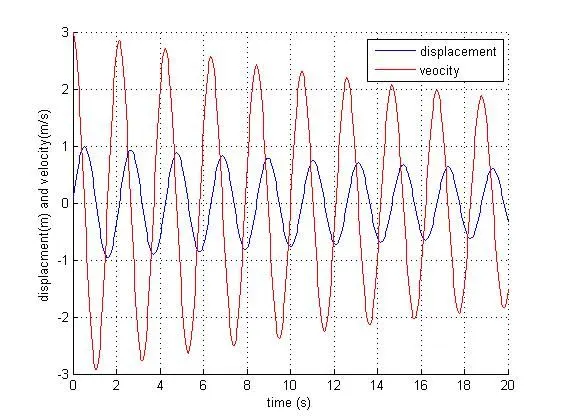
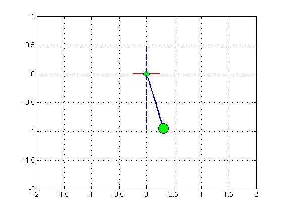
Next Animate the motion ,for that we need co-ordinate and theta . By using ouput value of the displacements we get that into the for loop that gives different theta for different value of displacements. then we define the co-ordinate as x0=0;y0=0;x1=l*sin(theta);y1=l*cos(theta);Then we plot figure 2 for animation pause function is used .for collecting the frame getframe function is used. and incrmental is used as 'd' that is initial =0 before the start of for loop

after the end for loop movie is made and save as MPEG-4 file with name pendulum motion. by using above mention function in the program.

Image of the ploting of pendulum:

link of the video :

https://www.youtube.com/watch?v=zptTuAnVYUc

This function is coded that define in ode45 as ode_func,

seond order ODE is made into first order and then calculate which give output as dtheta_dt.

function [dtheta_dt]=ode_func(t,theta,b,g,l,m)


theta1= theta(1);
theta2= theta(2);
dtheta1_dt = theta2;
dtheta2_dt = -(b/m)*theta2-(g/l)*sin(theta1);

dtheta_dt = [dtheta1_dt ; dtheta2_dt];

end

conclsion :

Here we have the damped motion of pendulum with respect to the time.