Week 3 - Solving second order ODEs

Objective: 1. Write a program that solves the equation of motion of a simple pendulum with damping using the ODE45 command.

2. Find the output values of angular displacement and angular velocity of a pendulum as a function of time.

3. simulation of the motion of the pendulum between 0 to 20 seconds.

4. Animation of the pendulum motion.

Theory: Consider a pendulum that consists of a ball and a rod. The rod is fixed at one end and from another end pendulum is free. At the initial position, the pendulum is at rest and we give a force of initial velocity of 3m/s.

The motion of the pendulum depends on Newton's second law. After the solving of Newton's equation of motion, we got a differential equation for the motion of the pendulum.

The differential equation is;

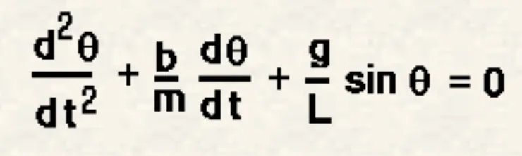
In the above equation,

g = gravity in m/s2,

L = length of the pendulum in m,

m = mass of the ball in kg,

b=damping coefficient.

The given values are;

L=1 metre,

m=1 kg,

b=0.05.

g=9.81 m/s2.

Solution:

First of all, convert the 2nd order differential equation of motion into the 1st order differential equation, so we can solve the 2nd order differential equation in MATLAB.

Let's assume,

theta = theta1

dtheta/dt = dtheta1/dt = theta2

d^2theta/dt^2 = d(dtheta1/dt)/dt = d(theta2)/dt

Now put all the values in the differential equation,

d(theta2)/dt+(b/m)*theta2+(g/L)*sin(theta1) = 0

d(theta2)/dt = -(b/m)*theta2-(g/L)*sin(theta1)----------(1)

dtheta/dt = theta2------------(2)

so now make the values of equation 1st and 2nd in a matrix form because we want every value of angular displacement and angular velocity at every value of time.

[theta1;theta2] = [theta2; -(b/m)*theta2-(g/L)*sin(theta1)]

Program of motion of pendulum:

Coding of function differential equation:

function [dtheta_dt] = ode_func(t,theta,b,g,l,m)


theta1 = theta(1);
theta2 = theta(2);

dtheta1_dt = theta2;
dtheta2_dt = (-b/m)*theta2-(g/l)*sin(theta1);

dtheta_dt = [dtheta1_dt;dtheta2_dt];


end

Explaining of code:

here we create functions for a differential equation that are in matrix form using function command.

we did so that we can get every value of angular displacement and angular velocity at every value of time.

we assume [theta1;theta2] as theta and then create variables theta1 and theta2 for both rows as theta(1) and theta(2) respectively.

In the theta1 variable, we got the 1st-row value of matrix form and in the theta2 variable, got the 2nd-row value.

In the function we used [dtheta_dt] = ode_func(t, theta,b,g,l,m), where ode_func is the name of a function, we have to write function name as file name should same and ''dtheta_dt'' is return output, ''t, theta,b,g,l,m'' are inputs.

Coding for plot angular displacement, angular velocity vs time, and plot of animation of the motion of a pendulum.

Explanation of coding:

clear all
close all
clc

% Inputs
b =0.5;
g =9.81;
m = 1;
l =2;

% solving 2nd ODE 

% Intial conditions of angular displacement and angular velocity
theta_0 = [0;3];   

% time points
t_span = linspace(0,20,500); 


% solving ODE

[t,result] = ode45(@(t,theta)ode_func(t,theta,b,g,m,l), t_span,theta_0);
figure(1)
plot(t,result(:,1))
hold on
plot(t,result(:,2))


xlabel('time')
ylabel('displacement,velocity')
legend('Angular Displacement','Angular velocity')
grid on

angular_displacement = result(:,1);


%  for loop for animation of pnedulum
ct = 1;
for i = 1:length(angular_displacement)
    
    ang_dis = angular_displacement(i);
    
     x0 = 0;
     y0 = 0;
     
     x1 = l*sin(ang_dis);
     y1 = -l*cos(ang_dis);
   figure(2)
   
     plot([x0 x1],[y0 y1],'color','b','linewidth',3);
     hold on
     plot([-0.5 0.5],[0 0],'color','g','linewidth',5);
     hold on
     plot(x1,y1,'o','markersize',20,'markerfacecolor','r');
     hold off
     axis([-4 4 -4 4]);  
     pause(0.001);
     M(ct) = getframe(gcf);
     ct = ct+1;

end

movie(M);
videofile = VideoWriter('pendulum.avi','uncompressed AVI');
open(videofile);
writeVideo(videofile,M);
close(videofile)

1. use % sign to write the comments in MATLAB.
   1. write all the input values of gravity, the mass of the pendulum, damping constant, and length of the pendulum.
   2. write initial conditions of the pendulum of angular displacement and angular velocity.
   3. The angular displacement of the pendulum is zero and angular velocity is 3m/s when time is 0 sec.
   4. we want to simulate the motion of the pendulum between 0 to 20 seconds, so used linspace command which gives the fixed value of time between 0 to 20 seconds of certain no. of values. The syntax of the command is linspace(initial value, end value, no. of values).
2. solve the differential equation using the ODE45 command and the syntax of t,result = ODE45 is ODE45(@(ode_func,tspan, initial conditions) where t is time and result that we want to output. ode_func is the function name, tspan is the time from initial to end value, initial condition. from this, we got the value of angular displacement and angular velocity for every value of time.
3. Now further, make plot angular displacement, angular velocity vs time using plot command on one graph using hold on command.
4. create for loop for animation of pendulum.
5. let's create a variable angular_displacement = result(:;1), which means that we got the output of angular displacement values.
6. create variable i for for_loop and the syntax of for-loop is i = 1:length(angular_displacement), which gives us all values of angular displacement.
7. make a variable ang_dis = angular_displacement(i), which gives a single angular displacement value one by one because we want x1,y1 value at every angular displacement.
8. Now get all the x1,y1 values of the moving pendulum.
9. further, makes all plots for animation of the pendulum.
10. here we used ct = 1 before for loop that means is the count of the frame of a position of the pendulum.
11. create M named variable and get all frames of all position of the pendulum using getframe command and the syntax is M(ct) = getframe(gcf) , which means that all frames will get in a single frame. gcf stands for get current frame. After that use ct = ct+1,i.e getting next frame if we put ct =1, so we get 500 frames in array for.
12. Now create a movie of all frames using the movie command.
13. Create a variable videofile and write a video from array data of frames using the VideoWriter command and the syntax is VideoWriter(file_name, profile).
14. open(videofile): opens the file associated with videofile for writing. When you open the file, all properties of the object become read-only. open discards all existing contents of the file.
15. writes data from an array to the video file associated with videofile, using videoWrite command and the syntax is videoWrite(videofile,array of frames).
16. close(videofile): closes the video file associated with videofile. You must call close to ensure that all data is written to the file.

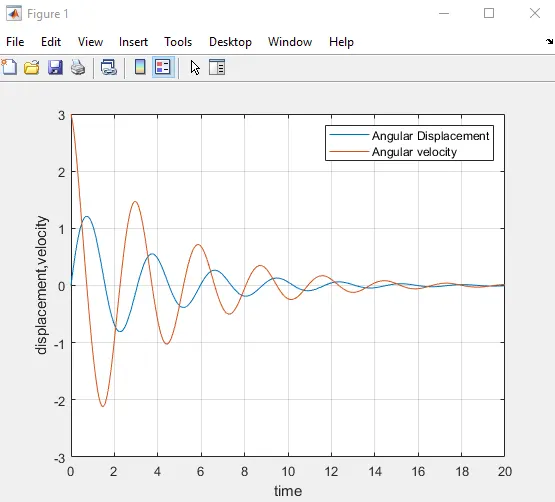
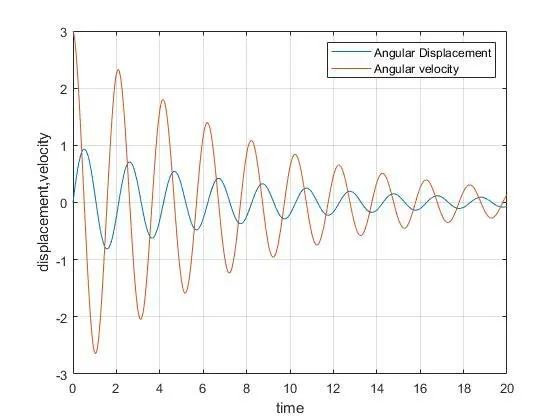
The plot of angular displacement, angular velocity vs time graph.

Youtube link for a video animation of the pendulum:

https://youtu.be/lvTaaxdFO-Y

Errors:

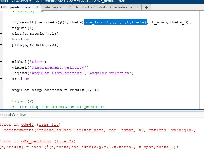
I just write t, theta and I got an error which showed that the same function handle terms will write in ode45 syntax. so i took help from the help documentation of ode45.

i got a different plot from the error.