Week 3 - Solving second order ODEs

AIM:

Write a python program to simulate the motion of pendulum between 0-20 sec. Also, this is to be shown using an animation of the same pendulum.
Here the following initial conditions are to used:

L (Length of the string) = 1 metre
m (mass of bob) = 1 kg
b (Damping Coefficient) = 0.05
g (Acceleration due to Gravity) = 9.81 m/`s^2`
s (Angular Displacement) = 0
`omega` (Angular Velocity) = 3 rad/sec at time = 0

THEORY:

Simple Pendulum : A simple pendulum is one which can be considered to be a point mass suspended from a string or a rod of negligible mass. It is a resonant system with a resonant frequency. Here the angle made by the string with the normal situated at the fixed end of the string is the angle `theta` and the if the length of the string and the displacement made by the bob is known, this angle `theta` can be evaluated using the formula : s = r * `theta`; where r is nothing but the length of the string and s is the displacement. From this, we can further find out the coodinates of the bob for certain time steps and plot for all these time steps. This can be done by using the resolution of vectors method.

Here the ODE representing the motion of a simple pendulum with damping is as below
`(d^2theta)/(dt^2) + (b/m)(d theta)/(dt) + (g/L)sin theta = 0`

To solve the above second order ODE, lets say that `theta = theta_1`
Thus, `(d theta)/(dt) = (d theta_1)/(dt) = theta_2` -------------------- (1)

With this we can write the above ODE as below,
`(d theta_2)/(dt) + (b/m)theta_2 + (g/L)sin theta_1 = 0` -------------------- (2)
here, the two first order ODEs obtained represent displacement and velocity respectively. This will be used in our program to evaluate the value of displacement and velocity at different time steps during the period of simulation.

CODING APPROACH:

Here, we will have to evaluate the displacement and velocity at different time steps. This can be done by solving the above first order ODEs using the function odeint from scipy module. After this we can use the above mentioned formula for the displacement of the simple pendulum to calculate the angle `theta`. For each value of `theta`, we need to evaluate the coodinates of the bob, which can be done using for loop. By plotting these coordinates along with coordinates of the fixed point, we get a series of plots which after stitching together result into a gif file.

ERRORS WHILE CODING:

The values generated when the model function is called, we had to extract the values for displacement which were in the matrix form. Here I used the statement - disp_values.append(theta[:,0]). This further resulted in a TypeError : only integer scalar arrays can be converted to scalar index. This was because, when the above statement was executed, disp_values contained an array of size 1. This was supposed to be 300. So, after realizing this, I used disp_values=(theta[:,0].tolist()), which extracted the items of the array as per requirement.

CODE:

import math
from scipy.integrate import odeint
import matplotlib.pyplot as plt
import numpy as np

# inputs
b=0.05
g=9.81
l=1
m=1
x0=0
y0=2

def model(theta,t,b,g,l,m):
	theta1=theta[0]
	theta2=theta[1]
	dtheta1_dt=theta2
	dtheta2_dt=-(b/m)*theta2-(g/l)*math.sin(theta1)
	dtheta_dt=[dtheta1_dt, dtheta2_dt]
	return dtheta_dt

#initial condition i.e. [displacement and velocity]
theta_0=[0,3]

# time points
t=np.linspace(0,20,300)
ct=0
# solve ODE
theta=odeint(model,theta_0,t,args=(b,g,l,m))
disp_values=[]
angles=[]
disp_values=(theta[:,0].tolist())
for i in disp_values:
	angles.append(math.radians(i))
#print(angles)

# Plot variation with time (displacement and velocity)

plt.figure()
plt.plot(t,theta[:,0],'b-',label=r'$\frac{d\theta_1}{dt}=\theta2$')
plt.plot(t,theta[:,1],'r--',label=r'$\frac{d\theta2}{dt}=-\frac{b}{m}\theta_2-\frac{g}{L}sin\theta_1$')
plt.ylabel('Plot')
plt.xlabel('time')
plt.legend(loc='best')
plt.show()

# Producing images for gif file
for i in angles:
	
	x1=l*math.sin(i)
	y1=l*math.cos(i)
	ct+=1
#	print(x1,y1)

	filename='test'+str(ct)+'.png'
	plt.figure()
	plt.xlim([-0.5,0.5])
	plt.ylim([0.8,2.1])
	plt.grid()
	plt.plot([-0.4,0.4],[2,2],linewidth=10)
	plt.plot([x0,x1],[y0,y1],linewidth=3)
	plt.plot(x1,y1,marker = 'o')
	plt.savefig(filename)

RESULTS:

https://drive.google.com/file/d/1aR8mtJ0EcUSDY26NBK3oJDTYPjBL-Aow/view?usp=sharing

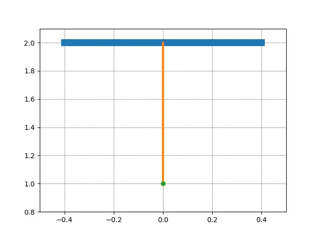
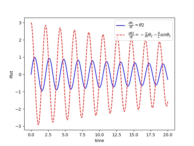
Above is the animation and plot for the displacement and velocity, obtained for the motion of a simple pendulum for the given conditions.