Week 3 - Solving second order ODEs
MAIN PROGRAM
%Solving second order ODE of a pendulum
clear all
close all
clc

%inputs
b = 0.05;
g = 9.81;
l = 1;
m = 0.1;

% initial condition
theta_0 = [0;5]

% time span
t_span = linspace(0,20,600)

% solving ODE
[t,results] = ode45(@(t,theta) ode_func(t,theta,b,g,l,m),t_span,theta_0);

%plotting
figure(1)
hold on
plot(t,results(:,1))
plot(t,results(:,2))
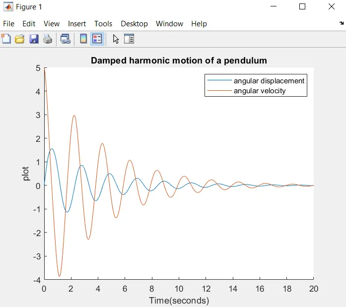
title('Damped harmonic motion of a pendulum')
legend('angular displacement','angular velocity')
ylabel('plot')
xlabel('Time(seconds)')

%for loop

ct = 1;
for i = 1:length(results(:,1))
    X0 = 0;
    Y0 = 0;
    X1 = 1*sin(results(i,1));
    Y1 = -1*cos(results(i,1));

    % plotting the animation
    figure(2)
    plot([-1 1],[0 0],'linewidth',5)
    axis([-2 2 -2 2]);
    hold on
    plot([X0 X1],[Y0 Y1],'linewidth',3)
    hold on
    plot(X1,Y1,'o','markersize',20,'markerfacecolor','y')
    title('Animation of transient behavior of a pendulum')
    axis([-1.5 1.5 -1.5 1])
    pause(0.01)
    hold off

    M(ct) = getframe(gcf)
    ct = ct+1

end

%storing the videofile in avi

movie(M)
videofile = videowriter('Pendulum Animation.avi','uncompressed avi')
open(videofile)
writevideo(videofile,M)
close(videofile)
EXPLANATION OF THE PROGRAM
1) The command clear all, close all, clc will clear the command window and all.
2) The inputs and variables are defined.
3) Then the initial conditions, angular displacement and angular velocity have been defined.
4) Timespan also have been defined.
5) To solve ODE, ode45 was used, it is a function in matlab used that solves ordinary differential or partial equation using a numerical method. The function ode45 takes 3 inputs. The three inputs are function to be integrated, the time span and the initial conditions [t,results] that the results have been calculated with respect to time.
6) After calculating the results, the plot command is used to plot the values. The graph contained two plots, one for angular displacement with respect to time and angular velocity with respect to time.
7) The axis labels are also defined.
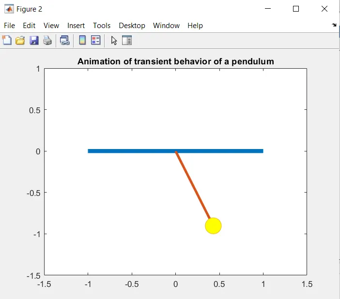
8) The pause command was used to pausing the command for certain time, for this program the pause of 0.01 was used.
9) the final step of the variable is to add a +1 in the ct variable, this will increment the frame every time for the loop run.
10) The end command is used for the plot and for the loop to stop both from running.
11) The video writer command is used to create a animation or video in the given avi format.
OUTPUT :
SUB PROGRAM
%A function program which will be called in the main program

function[dtheta_dt] = ode_func(t,theta,b,g,l,m)
theta1 = theta(1)
theta2 = theta(2)
dtheta1_dt = theta2
dtheta2_dt = -(b/m)*theta2 - (g/l)*sin(theta1)
dtheta_dt = [dtheta1_dt; dtheta2_dt]
end
EXPLANATION OF THE SUB PROGRAM
1) A function is a group of statement that perform a task together.
2) The name of the file and function should be same.
3) Functions operate on variables within their own workspace.
4) The function is called in the main program.
OUTPUT :
ERRORS FACED WHILE PROGRAMMING
1) Unrecogonised function or variable X_start while plotting.
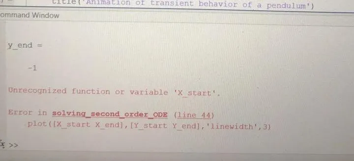
I have overcome the error by defining the variable.
GOOGLE DRIVE LINK
https://drive.google.com/drive/folders/12YBLdLNOVjfLyl4GX3l2sfWSoMIec3GH?usp=sharing