Week 3 - Solving second order ODEs

Project:-- To make program in PYTHON to solve the ODE of damped SHM of simple pendulum & to create animation of the SHM.

Objective of the project:-- Plotting the angular velocity & angular displacement with respect to time for damped simple harmonic motion of simple pendulum with the help of data obtained by solving the ODE of the damped SHM & using these information creating animation of the damped SHM. All these are to be done by making a program in PYTHON.

Theory:--

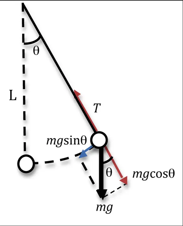
The motion of the simple pendulum is simple harmonic motion. Here force component F=mg.sin(theta) plays as restoring force & it is always directed towoards equilibrium point of the path of the bob of simple pendulum, where theta is angle between the string of the pendulum & the vertical axis passing through the point of the suspension. The restoring force F is dircetly propotional to the displacement of the bob at that moment. If the motion is free , the pendumlum oscilates for ever with the amplitude unchanged. But in damped motion there is resistive force which is propotional to the instantenious velocity the the bob of the pendulum. In case of damped motion the angular displacement & velocity are diminished with time & the motion comes to rest finally..

The equation given below is an Ordinary Differential Equation (ODE) which is a 2nd order equation with two variables, theta & t. This is the ODE of damped motion of simple pendulum.

`(d^2theta)/dt^2+(b/m)(d theta)/(dt)+ (g/L)Sintheta=0`

Here theta is angular displacement , t is time, b is damping co efficient, m is mass of bob, g is accelaration due to gravity & L is effective length of simple pendulum

Brief discussion of the project:-- To solve the ODE the solver 'odeint' is used in the program in PYTHON. The initial input is L=1metre, m=1kg, b=0.05, g=9.81m/s2. We have to simulate the motion in time span of 0 to 20 sec. Initial angualr displacement is 0 & initial angular velocity is 3 rad/sec at t=0.

Here from the 2nd order ODE, two 1st order ODEs are made.

Let `theta=theta1; (d theta)/dt=(d theta1)/dt;` Let `(d theta1)/(dt)=theta2; (d^2theta1)/(dt^2)=(d theta2)/(dt)`

So using above relation for the ODE of damped motion of Simple pendulum we get

`(d theta2)/(dt)+(b/m) theta2+(g/L)Sin theta1=0`

So `(d theta2)/(dt)=-(b/m)theta2-(g/L)Sin theta1`-----1 & `(d theta1)/(dt)=theta2`----2

These two differential equations of 1st order can be expressed in matrix form like below

`d/dt[theta1;theta2]=[theta2; -(b/m)theta2-(g/L)Sin theta1]`

`[theta1; theta2]`is solution vector. Let `theta=[theta1;theta2]`. So we can say that `theta(1)=theta1` & `theta(2)=theta2`

So the matrix form of 1st order ODE as explained above is given as input to the solver 'odeint' used in the program.

The solver actually does the definite inetegration & give solution vector `[theta1;theta2]`which is a matrix containing angular dispalcement & angular velocity for 200 instant in the time span 0 to 20 sec in two columns.

These angular displacement & angular velocity are plotted with respect to time.

These data are used to create animation of the damped motion of Simple pendulum.

Below the code in PYTHON to solve the ODE & to plot the angular velocity & displacement w.r.t time are given below.

# program to solve ODE & ploting angular displacement & velocity with time

import math
import numpy as np 
import matplotlib.pyplot as plt 
from scipy.integrate import odeint

#Function that returns ODE in matrix form

def model(theta,t,b,g,l,m):
	theta1=theta[0]
	theta2=theta[1]
	dtheta1_dt=theta2
	dtheta2_dt=-(b/m)*theta2-(g/l)*math.sin(theta1)
	dtheta_dt=[dtheta1_dt, dtheta2_dt]
	return dtheta_dt

b=0.05
g=9.81
l=1
m=1

# initial condition
theta_0=[0,3]

# time array

t=np.linspace(0,20,200)

# solve ODE
theta=odeint(model,theta_0,t,args=(b,g,l,m))
print(theta[:,0])
print(theta[:,1])

# plot result

plt.plot(t,theta[:,0],'b-',label= 'Angular Displacement')
plt.plot(t,theta[:,1],'r--',label='Angular Velocity')
plt.ylabel('Plot')
plt.xlabel('Time')
plt.legend(loc='best')
plt.show()

Explanation of code:-- First math, numpy, pyplot, scipy module are imported for mathemetical calculation, for using linspace command , for plotting, for using solver 'odeint' respectively.

Then a function called 'model' is defined where two 1st order ODEs are created fron the 2nd order ODE & the two 1st order ODEs are represented in a matrix form. When the function is called by the solver, this matrix as an out put of the function is used as input by solver.

Initial values of b, g, l, m are declared which are used as input by the solver 'odeint'.

Then the initial condition of angular displacement & angular velocity which are 0 & 3rad/sec respectively are declared in a matrix form theta_0[].This initial condition is used by the solver 'odeint'

The time span 0 to 20 sec is divided in to 200 equal instant by using linspace command, which are used by solver & also used during ploting angular displacement & velocity w.r.t time.

Then the ODEINT solver is used to solve the ODE which is sent to it in a matrix of two 1st order ODEs by calling the function 'model'. Besides this as input b,g,l, m & time span are given to solver.

The output of the solver (after solving the ODE given to it) is stored in the varriable theta in a matrix form. theta[:,0] gives angual displacements for 200 instant in the time span 0 to 20 sec & theta[:,1] gives angular velocity in the same way.

After that, the code is written for plotting the angular displacement & angular velocity with respect to time with proper legend , proper X & Y axis label.

The plot obtained by running the program is given below.

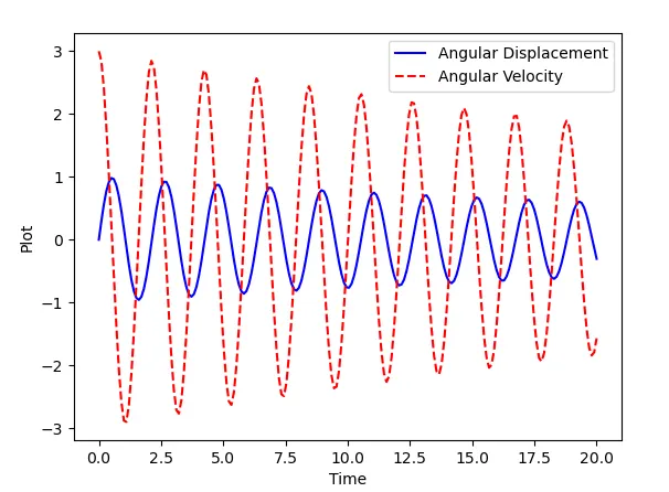
From the above plot we can understand that, the SHM is an damped motion. Due the presence of the resistive force the maximum values of angular displacement & angular velocity are diminishing with time. After some times these will become zero. We can also see from the plot that when the angular displacement is at maximum , the angular velocity is at minimum (=0) & vice versa. At starting when the angular velocity is 3rad/sec, the angular displacement is zero.

The program to create the animation of the damped SHM of the simple pendulum , using the output of the solver is given below.

# Program to create animation of SHM
import math
import numpy as np 
import matplotlib.pyplot as plt 
from scipy.integrate import odeint

#Function that returns ODE in matrix form

def model(theta,t,b,g,l,m):
	theta1=theta[0]
	theta2=theta[1]
	dtheta1_dt=theta2
	dtheta2_dt=-(b/m)*theta2-(g/l)*math.sin(theta1)
	dtheta_dt=[dtheta1_dt, dtheta2_dt]
	return dtheta_dt

b=0.05
g=9.81
l=1
m=1

# initial condition
theta_0=[0,3]

# time array

t=np.linspace(0,20,200)

# solve ODE
theta=odeint(model,theta_0,t,args=(b,g,l,m))
d=theta[:,0]
print(theta[:,0])
print(theta[:,1])

#Origine
O1=0
O2=0

# Loop for animation

ct=1

for i in d:
	C1=l*math.sin(i)
	C2=-l*math.cos(i)
	

	filename=str(ct)+'.png'
	
	plt.figure()
	plt.plot([O1,C1],[O2,C2],'b',linewidth=5)
	plt.plot(C1,C2,'o',markersize=20,color='r')	
	plt.xlim([-1,1]) 
	plt.ylim([-1.5,0.2])
	plt.savefig(filename)
	ct=ct+1

Explanation of code:--

Here like privious program, the required modules are imported, the function 'model' is defined, then value of b,g,l,m are declared, after that initial condition ( at t=0) of angular displacement & angular velocity are declared. Then the the time span of 0 to 20 sec is divided in 200 instant by linspace comand. The the solver 'ODEINT" is called to solve the ODE.

The the out put of the solution of ODE given by the solver is used to create the animation.

At first the co ordinate of the point of suspention of the simple pendulum is declared as (0,0) in the variable (O1,O2).

Then a loop has been created to create the animation.

First a counter ct is declared with its initial value as 0.

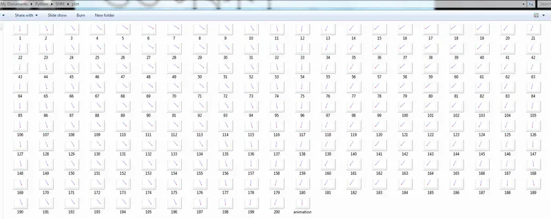
Then a for loop is created with the help of the column matrix d=theta[:,0] which is the matrix of angular displacement at 200 instant in the time span of 0 to 20 sec. For that 200 instant, the postision of the centre of the bob is defined with this for loop. Then within the loop for every instant picture of the simple pendulum is craeted & the picture is saved as a filename created by the value of the counter at that moment with extention.png. In this way total 200 no of files are saved for different position of the pendulum for 200 instant for time duration 0 to 20 sec for the oscilation of the pendulum.

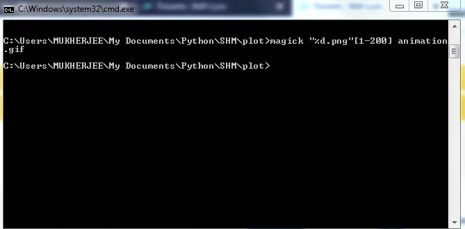
Then in the command prompt, within the proper directory. the following command is used to stich the 200 .png files to form the animation. For the animation the file 'animation.gif' is created.

The photographs taken by snipping tool, for the command used in the command prompt & 200 files saved for different postition of pendulum are given below.

The Google drive link for the animation file of animation.gif, is given below.

Damped motion of Simple Pendulum

From the animation it is clear, that the SHM of the simple pendulum is damped motion due to exsistance of resistive force (damped coefficient b =0.05) because of that the amplitude of the oscilation is diminishing.