Project on Optimization of Stalagmite Function by Genetic Algorithim.

Project on Optimization of Stalagmite Function by Genetic Algorithim.

Aim of the Project:-- Wiriting code in Matlab to find out global maxima of Stalagmite Fuction by Genetic algorithim. Finding statistical behevior of GA in three different cases, 1) With unbound inputs & increased iteration, 2) with bounded input & 3)with incresing population & bounded input .

Mathemetical form of Stalagmite function:--

Stalagmite Function =f(x,y)

f(x,y)=f1(x).f1(y).f2(x).f2(y)

Where

f1(x)=[sin(5.1.Π x+0.5)]⁶

f1(y)=[sin(5.1.Π y+0.5)]⁶

f2(x)=exp[-4.ln(2).{(x-0.0667)²/0.64}]

f2(y)=exp[-4.ln(2).{(y-0.0667)²/0.64}]

Genetic Algorithim:--

Genetic Algorithim (GA) is a method by which a optimization problem (objective function) can be solved on the basis of biological evaluation theory proposed by Charls Darwin. GA is random based Evaluation Algorithim. GA works on a population which consists of no. of solutions.Each solution is an induvidual. Induviduals in a population are selected randomly.Each induvidual has a chromosome. Each chromosom has a set of Genes. Each gene is represented by digit of binanary, octal etc number . For example 1110 is a chromosome of a induvidual. 1,1,1,0 are gene on that chromosome. Suppose 1110, 1010, 1001 are the induviduals of a population. GA bigens work on a randomly selected initial population. Each induvidual of a population has a fitness value. Fitness value is calculated by fittness function. Higther is the fitnes value, better is induviduals. In this way best induviduals are selected based on threshold-fitness values.These selected induviduals forms mating pool. Induviduals in the mating pool are called parents. Every Two parants randomly or sequencially selected, generates offsprings (children). Here offsprins are generated by two method,which are crossover & mutation. The children generated forms a new population, which replaces the previous population. Each population is called a generation.These children are called induvidual of the new generation. Again from the new generation bests induviduals are selected to form next generation. In this ways by generating successive generation , the optimised solution is found out.

GA can be summarized by the following way.

1.Initial Population--2. Fitness calculation--3.Mating pool--4.Parents selection---5.Mating(crossover, mutation)--6.Offsprings(forms next generation).

In crossover genes of offsprins of new generation consists of genes both parents.

In mutation, gene of offspring is changed randomly to give it a new property which is not inherrited from parents.

Besides this an induvidual having very good fitness value can passed to next geration without any change as elite child.

Plotting Stalagmite function with Optimised value given by GA:--

Matlab gives a solver called 'ga' which finds minimum value of objective function using genetic algorithim.

Simplest syntax of ga is

[x, fval]=ga(fun,nvars)

where 'ga' is solver, 'fun' is objective function which is called here, 'nvars' are number of input variables, 'x' is the best individual found after optimization, faval is best optimaised value against the best induvidual of final generation.

So 'fval' is minimum value of the objective function.

One important point is , as Genetic Algorithim is stochastic , it chooses randomly, every time ga runs it will give different results each time.

Code(in MATLAB) of Stalagmite Function, & runing 'ga' with the stalagmite function as objective function.

% Code of Stalagmite Function

function fn= stalagmite(input_vector)
x=input_vector(1);
y=input_vector(2);

f1=(sin(5.1*pi*x+0.5)).^6;

f2=(sin(5.1*pi*y+0.5)).^6;

f3=exp(-4*log(2)*((x-0.0667).^2/0.64));

f4=exp(-4*log(2)*((y-0.0667).^2/0.64));


fn=(f1*f2*f3*f4);

end




%Code for Runing 'ga' & ploting stalagmite function & find out put of 'ga'.
clear all
close all
clc

% Defining search place   % [One dimensional array of x & y are declared having limit 0 to                                                                      
x=linspace(0,0.6,150);    % 0.6 & 150 elements owithin it.]
y=linspace(0,0.6,150);

[xx,yy]=meshgrid(x,y);  %[Two dimansional array xx & yy are created with meshgrid function]

% Evaluating Stalagmite Function;  %stalagmit function is evaluated using a for loop 
   for i=1:length(xx)                   
     for j=1:length(yy)
     input_vector(1)=xx(i,j);
     input_vector(2)=yy(i,j);
     f(i,j)=stalagmite(input_vector);
     end
 end 
 
 [input, fval]=ga(@stalagmite,2);  %['ga' solver use function handelar @stalagmite 
                                  %'ga' takes two input varriables as x & y & gives minimum
 Output = fval                    % value of function as 'fval' & best induviadual as Xval,   
 Xval=input(1)                    % Yval]
 Yval=input(2)
 
 
 figure(1)                         % [One figure is created inwhich two subbplots is crated
 subplot(2,1,1)                    % 1st subplot gives plot (smooth) of stalagmite functiom
 surfc(xx,yy,f)                    % 2nd subplot shows minimimum value generated by'ga'with 
 shading interp                    % respect to the the stalagmite function]
 title('stalagmite function')
 subplot(2,1,2)
 hold on
 surfc(xx,yy,f)
 shading interp
 plot3(Xval,Yval,fval,'color','b','marker','o','markersize',5,'markerfacecolor','r')
 grid on
 title('stalagmite function with optimized value of the function given by GA')

Result of the runing 'ga'

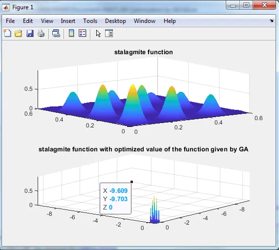
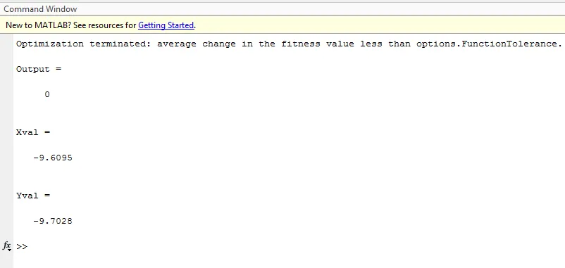
Here we can see the minimum value (out put/fvalue) which is given by 'ga' is 0 & at the point (-9.6095,-9.7028). Here we can see that the minimum value is at distant from the stalagmite function. So here the performance of 'ga' is not at all satisfectory. But here 'ga' runs just one time.

So this is in nutsell, how 'ga'works using Genetic Algorithim.

But as per challange given, we have to find out Global maximum value of stalagmite function using Genetic Algorithim solver 'ga'.

For this we have to change in coding of stalagmite function which is given below.

% Modified coding of Stalagmite function

function fn= stalagmite(input_vector)
x=input_vector(1);
y=input_vector(2);

f1=(sin(5.1*pi*x+0.5)).^6;

f2=(sin(5.1*pi*y+0.5)).^6;

f3=exp(-4*log(2)*((x-0.0667).^2/0.64));

f4=exp(-4*log(2)*((y-0.0667).^2/0.64));


fn=-(f1*f2*f3*f4); %['-' sign has been incorporated]

end

For getting maximum value of the stalagmite function, in the code of the stalagmite function '-' sign is incorporated as 'fn=-f1*f2*f3*f4' to pass pass the stalagmite function in inverted manner so that 'ga' finds minimum value when it will pick up the peak of the function. So the peak will be in -ve sign.

Case 1:-- Statistical behevior of 'ga' with increased iteration & unbounded input to 'ga'

Code for runing 'ga' with modified stalagmite function

clear all
clc

% Defining search place

x=linspace(0,0.6,150);
y=linspace(0,0.6,150);

iteration=50;

% Creating 2-dimensional mesh
[xx,yy]=meshgrid(x,y);

% Evaluating Stalagmite Function
 for i=1:length(xx)
     for j=1:length(yy)
     input_vector(1)=xx(i,j);
     input_vector(2)=yy(i,j);
     f(i,j)=stalagmite(input_vector);
     end
 end
 f=-f; 

 % Study_1, Statistical bihavior of GA with unbound input
tic; 
 for k=1:iteration     
     [inputs, fopt(k)]=ga(@stalagmite,2);
     xopt(k)=inputs(1);
     yopt(k)=inputs(2);     
 end
 fopt=-fopt;
 fopt
 study_1_time=toc
 
 figure(1)
 subplot(2,1,1)
 hold on
 surfc(x,y,f)
 shading interp
 plot3(xopt,yopt,fopt,'color','b','marker','o','markersize',5,'markerfacecolor','r')
 title('unbound input')
 subplot(2,1,2)
 plot(fopt,'color','b','linewidth',1)
 xlabel('iteration');
 ylabel('Function Maximum');

So during ploting to prsent the the function in right way(not inverted) & to show the max value in +ve sign in the code following steps are used

f=-f (to plot the function in right way)

fopt=-fopt (to plot max values in +ve sign)

Increase of iteration of 'ga':--

Here no. of iteration of the solver 'ga' is increased to 50 from the 0 of the previous case by using a 'for loop' with varrying the value of variables 'k' from 1 to 50. No. of iteration is stored in the variables 'k'. For every iteration of 'ga', the max value of the objective function is stored in the row vector 'fopt'. For every element of 'fopt', value of individuals are stored in the row vectors 'xopt' & 'yopt, through inputs(1) & inputs(2) respectively.

Significans of increasing the iteration of 'ga':--

By increasing the iteration, the chance of getting close to best optimised value or getting optimised value is increased. We can not trust the output of very few iterations for getting the optimised value. With increasing the no. of iteration of 'ga' solver, crossover, mutation are occured repeatedly, as a result chance of getting best optimised value is increased. Besided this with the incraese of no. of iteration the time taken for runing 'ga' is also incresed. So the no. of iteration should be incresed untill we are getting the steady state value (convergence of values towords the best optimised value).

Result of case 1

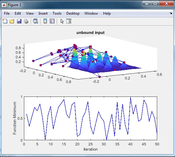
From the plot given above we find the max values (indicated by red marked point) of the stalagmite function predicted by 'ga' in each iteration in 3D view.

Here 'ga' works on unbound input of x & y & number of iteration is incresed to 50.

In the 2nd subplot max value predicted by ga is ploted with respect to no. of itaration.

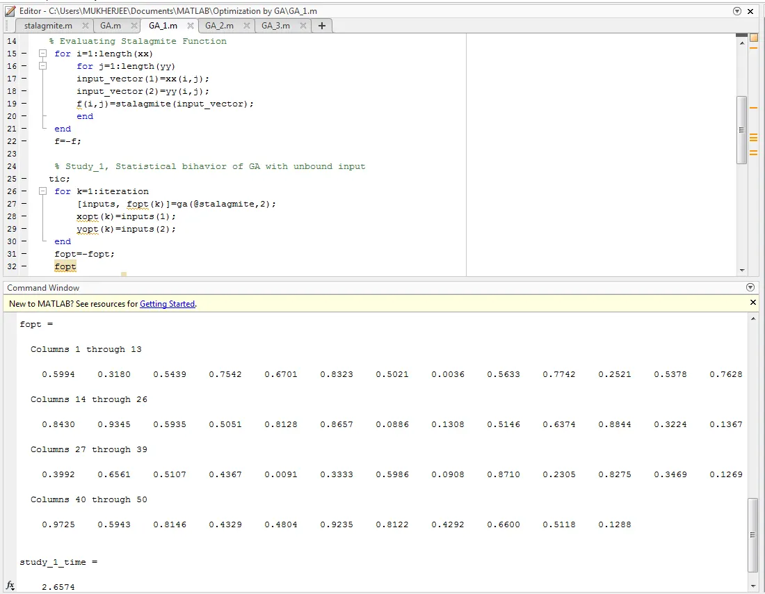
From the plot & result data given in command window we find that max value (based on all 50 iterations of 'ga') is 0.9725 & it is given by only one iteration (iteration no. 40th).

Other value close to max value, is 0.9345 for 15 th iteration. Max valuse given in other iteration of 'ga' is well below the 0.9345(which is maximum based on all iteration) As per plot many max values are very distant form the function. The performance of 'ga' is not satisfactory.

The time taken for runing 'ga' is 2.6574 sec. Some

Case 2:-- Statistical behevior of 'ga' with bounded input.

Code in MATLAB for runing the 'ga' solver with bounded input is given below.

% Code(in matlab) for running 'ga' with bounded input

clear all
clc

% Defining search place

x=linspace(0,0.6,150);
y=linspace(0,0.6,150);

iteration=50;

% Creating 2-dimensional mesh
[xx,yy]=meshgrid(x,y);

% Evaluating Stalagmite Function
 for i=1:length(xx)
     for j=1:length(yy)
     input_vector(1)=xx(i,j);
     input_vector(2)=yy(i,j);
     f(i,j)=stalagmite(input_vector);
     end
end
 f=-f; 
 % Study_2, Statistical bihavior with bounded input
 tic;
 for k=1:iteration    
     [inputs, fopt(k)]=ga(@stalagmite,2,[],[],[],[],[0;0],[0.6;0.6]);
     xopt(k)=inputs(1);   %[ bound of in put parameter is given as 0 to 0.6 for x & y]
     yopt(k)=inputs(2);     
 end
 fopt=-fopt;
 fopt
 study_1_time=toc
 
 figure(2)
 subplot(2,1,1)
 hold on
 surfc(x,y,f)
 shading interp
 plot3(xopt,yopt,fopt,'color','b','marker','o','markersize',5,'markerfacecolor','r')
 title('bounded input')
 subplot(2,1,2)
 plot(fopt,'color','b','linewidth',1)
 xlabel('iteration');
 ylabel('Function Maximum');

Here range of two input parameters passed to 'ga' solver is declared in the syntax of 'ga'. In this case the both input parameters (x & y) are bounded within range of 0 to 0.6. By declaring the bound of the input, we ensure that 'ga' randomly select induvidual within the range. As a result of this the solutions given by 'ga' are more converging towords the best optimised value & chance of getting best optimised value is incraesed. range of the inut variables are given on the basis of previoue iteration & knowledge of the objective function.

Result of Case-2:--

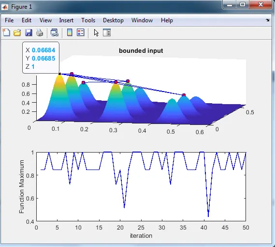
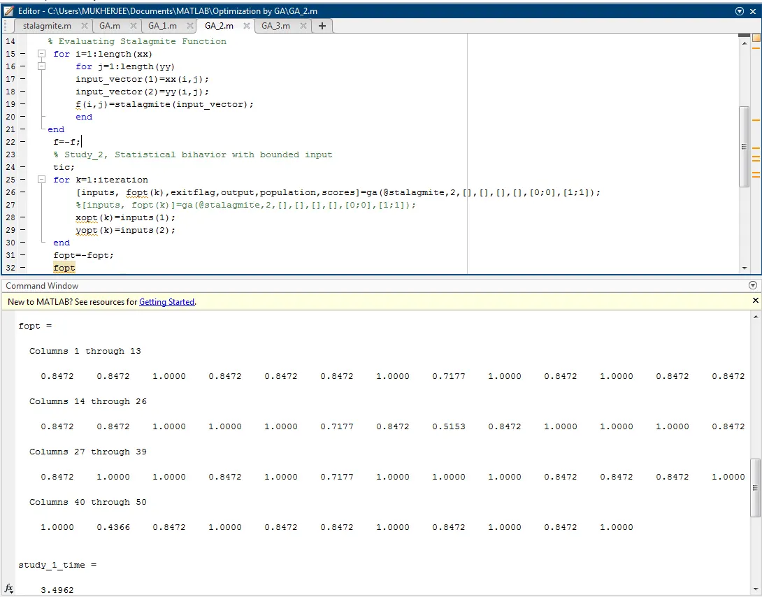
The subplot1 above, shows max values given by the 'ga' with the stalagmite function in 3d. Subplot2 gives plototing of max values with no. of iterations. From the above plot & data given by caommand window we can find that the max value of the objective function (stalagmite) as given by 'ga' is 1. Other max values (fopt) of the function for all iterations are more convereged to the max values 1. In 22 no. of occassions (iterations) 'ga' give the maximum values as 1.Besides this, in 23 occassion(iterations) 'ga' gives the best optimised value as 0.872. So in this case-2, performance of 'ga' is satisfactory than the previous case-1.

Time taken by ga to run is 3.4962sec.

Case 3:-- Statistical behevior of 'ga' with increasing population size.

By incresing population size, 'ga' works on more inuviduals. Due to this, chance of more good induvidusals getting selected on the basis of fittness function, is incraesed. Due to this, output data given by 'ga' are more converging towords the best optimised value. As a result of this, chance of getting best induviduals in more number, are increased. With this we can be conclusive with solutions given by 'ga' & get the best optimised value definitely.

Code (in MATLAB) for runing 'ga' with incraesed population size.

clear all
clc

% Defining search place

x=linspace(0,0.6,150);
y=linspace(0,0.6,150);

iteration=50;

% Creating 2-dimensional mesh
[xx,yy]=meshgrid(x,y); 

% Evaluating Stalagmite Function 
 for i=1:length(xx)
     for j=1:length(yy)
     input_vector(1)=xx(i,j);
     input_vector(2)=yy(i,j);
     f(i,j)=stalagmite(input_vector);
     end
 end
 f=-f; 
 % Study_3, Statistical bihavior(using bounded input,fixing PopulationSize) 
  options=optimoptions('ga','PopulationSize',150);  
 tic;      %[ In the syntax of 'ga' population size is declared as a option]
 rng default
 for k=1:iteration     
 [inputs, fopt(k)]=ga(@stalagmite,2,[],[],[],[],[0;0],[0.6;0.6],[],[],options);
  xopt(k)=inputs(1);
  yopt(k)=inputs(2);     
 end
 fopt=-fopt;
 fopt
 study_1_time=toc 
 
 figure(3)
 subplot(2,1,1)
 hold on
 surfc(x,y,f)
 shading interp
 plot3(xopt,yopt,fopt,'color','b','marker','o','markersize',5,'markerfacecolor','r')
 title('Bounded input with increased population')
 subplot(2,1,2)
 plot(fopt,'color','b','linewidth',1)
 xlabel('Iteration');
 ylabel('Function Maximum'); 

Here population size is incrased by passing a 'options' ' to the 'ga' solver. The 'options' is made by the function called 'optimoption'.

If no population size is declared, by default the 'ga' take 50 as population size. In the study Case-3, population size is declared as 150.

Result of Case-3 :--

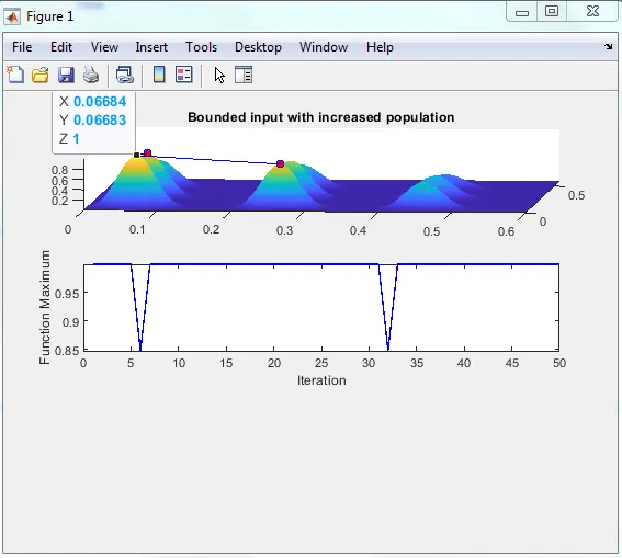
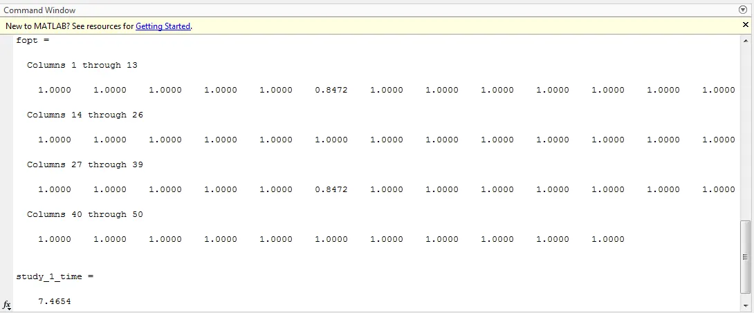
From the sub plot1 & 2 & data given by command window above, we find that all the optimised values for all 50 iterations, are converged to two values (fopt) of stalagmite function which are 1 & 0.8472. In only two occassion (iterations), 6th & 32nd no. of iteration the max value given by 'ga' is 0.8472 in all other iterations max value of the objective function are coming out as 1. So from here we can be conclude that the 'ga' solver gives rise to Global maximum value of stalagmite function as 1 by the nethod of Genetic Algorithim.

Here time taken by 'ga' to run is 7.4654 sec.

Reproducibillity of 'ga':--

'ga' makes random choice during selection of induvidual, in otherwords 'ga' is stocashtic in nature, so we get different results for every iteration of 'ga'. If we need to reproduce the result for every time we run the 'ga', we have to put the code 'rng default'. By using this code we ensure that 'ga' picks up same induviduals of initial population again & again when we run 'ga' repeteadly.

In our 'Case-3', the code 'rng default' has been incorporated just before the 'for loop' for the iteration of 'ga'. So for the code of in case3 we get same output with repeated iteration of 'ga'.

Explanation of Syntax of 'ga' :--

syntax of 'ga' is as follows.

[x,fval]=ga(fun, nvars,A,b,Aeq,beq,lb,ub,nonlcon,IntCon, options)

'x' is the value of best individual for the best optimised value.

'fval' is the best optimised value of objective function.

'ga' is a solver which find the minimum value of objective function.

'fun' function handeler of the obgective function.

'nvars' is the no of input variables passing to 'ga' solver.

A,b are the lenear non equality constarint passing as a in put to 'ga'

Aeq, beq are lenear equality constraint passing as a input to 'ga'.

lb,ub are lower bound & upper bound of input variables passing as input to "ga'.

'nonlcon' is non lenear constraint passing as input to 'ga'.

'options' is also a input to 'ga' .

Syntax of 'ga' can also be as follows'

when there is no leanear inequality,set A=[], b=[] ;

when there is no leanear equality,set Aeq=[], beq=[];

when no bound exsist, set lb=[], ub=[] ;

when there no non lenear constraint, set nonlcon=[];

when there is no IntCon, set IntCon=[];

In our case, in the code for Case-3, only bound of input & 'options' are passed as input to 'ga'.

According to that in our case the pattern of syntax of 'ga' becomes as given below,

[x, fval]=ga(fun,nvars,[],[],[],[],lb,ub,[],[],options);

Stopping criteria of ga:--

Followings are the some of stipping criteria 'ga' used for stopping.

1) Generations — 'ga stops if no. of generations becomes equal to maximum no. of Generation.

2)Time limit — When time taken by 'ga' to run crosses the time limit set it stops.

3) Fitness limit — When the algorithim does not find the fitness function value of best induvidual of current population,greter thanor equal to fitness limit.

4) Function tolerance — The algorithm stops the average relative change in the fitness function value is greater than Function tolerance.

In our Case-1, following are the causes of stooping the 'ga'

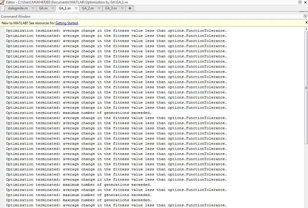
So from the data given in the command window , we find that point 1 & 4 are the stopping criteria in our case.