Project 2 - Rankine cycle Simulator
Project:-- Creation of Simulation of Rankine cycle using MATLAB.
Aim of the project:-- With the three input data (turbine inlet pressure,turbine inlet temperature & tubine outlet pressure), all the state points of Rankine cycle are to be defined. As out put, ploting of P-V diagram, T-S diagram & h-s diagram are to be shown. Besides this, Work done by turbine, Net Work done, Thermal efficiency of the rankin cycle, Specific-Steam-consumption are to be calculated & to be shown along with all state varriables, in comand window. All these are to be done by coding in MATLAB. The program only takes the above mentioned inputs & does all the required calculations & gives the above mentioned output. Here Steam table data (Xsteam library) given, is used to calculate state varriables & points inbetween state points.
Rankine Cycle:--
Rankine cycle is an ideal cycle for comparing performance of steam plants. It is modified form of Carnot cycle with steam as working substance,in which condensation process continued until the steam is condensed in to water completly.
The rankine cycle consists of following process.
1. Isentropic expansion of steam(Saturated/wet/superheated) in turbine/heat engine. Here pressure & temperature of steam falls & after expansion the steam may be dry or wet. Here work is done by turbine/Engine. Here we get mechanical work from turbine/ engine.
2. Condensation of steam coming out from turbine/engine into water is done by condenser. This is constant pressure & temperature process. Here latent heat of dry steam present, is rejected.
3. Condensed water from condenser is isentropically compressed to raise its pressure to boiler pressure & feeded in to boiler by feed pump. Work is done by feed pump . Here work is done by external agent on the system.
4. Heating of feeded water in side boiler at constant pressure to convert it in to wet/sturated/superheated steam as per requirement. Here heat is added in to system.
In this peroject we consider the super heated steam to be feeded in to turbine.
T-S diagram of The Raknine cycle with super heated stem of this project, is given below
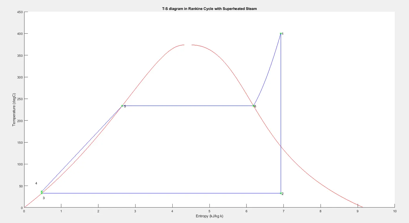
According to the T-S diagram given above , blue lines indicates the following process & red lines indicate the staurated liquid line & sturated steam line.
1-2--Isentropic Expansion of super heated steam in turbine.
2-3--Condensation of steam coming out from the turbine in to water by condenser.
3-4--Isentropic Compression of condensed water by feed pump
4-5--Heating of water at constant boiler pressure to convert it into sturated water
5-6--Heating of saturated water to convert it in to dry stuarted steam inside boiler at constant boiler pressure.
6-1--Super heating of steam at constant pressure.
Let H1, H2 & H6 are the enthalpy for steam for state points 1,2 & 6 respectively.
H3, H4, H5 are enthalpy of water at state points 3, 4 & 5 respectively.
Heat added during the cycle = H1-H4
Heat rejected during the cycle = H2-H3
feed pump work = H4-H3
Net workdone during cycle (W_net) = Heat added-Heat rejected = (H1-H4)-(H2-H3)=(H1-H2)-(H4-H3)=H1-H2-Wp
Rankine cycle efficiency = Net work done / Heat added = (H1-H2-Wp)/(H1-H4) = (H1-H2-Wp)/(H1-H3-H4+H3) = (H1-H2-Wp)/(H1-H3-Wp)
Sometimes pump work is neglected, then rankine Cycle efficiency = (H1-H2)/(H1-H3)
back work ratio = Pump work /Turbine work = Wp/(H1-H2)
Specific heat consumption (S.S.C) = It is specific rate of flow of steam. It is defined as mass of steam to be supplied to turbine/engine to produce unite amount of work. So S.S.C= 1kwh/W_net.
The code in MATLAB is given below.
%Rankine cycle with Super-heated steam

clc
clear all

% Input Data

%Turbine inlet pressure (in BAR)
P1=30;

%Turbine inlet temperature (in degC)
T1=400;

% Turbine outlet pressure (in BAR)
P2=0.05;


% state variable at point 1, (Turbine inlet point, super heated steam from boiler)
V1=XSteam('v_pT',P1,T1);
S1=XSteam('s_pT',P1,T1);
H1=XSteam('h_pT',P1,T1);


% state variable at point 2, (Turbine outlet point)
T2=XSteam('Tsat_p',P2);
Sg2=XSteam('sV_p',P2);
Sf2=XSteam('sL_p',P2);
Sfg2=Sg2-Sf2;
x=(S1-Sf2)/Sfg2;
S2=Sf2+x*Sfg2;

Hf2=XSteam('hL_p',P2);
Hg2=XSteam('hV_p',P2);
Hfg2=Hg2-Hf2;
H2=Hf2+x*Hfg2;
Vg2=XSteam('vV_p',P2);
V2=x*Vg2;

% PV^n=constant, finding value of n.
% P1*V1^n=P2*V2^n
n=(log(P2)-log(P1))/(log(V1)-log(V2));% value of 'n' is evaluated
C=P1*V1^n;
V_exp=linspace(V1,V2,100);
P_exp=C./(V_exp).^n;


% state variable at point 3,(State point after the steam from
% turbine,condensed in to water)
P3=P2;
T3=T2;
V3=XSteam('vL_p',P3);
Hf3=Hf2;  %(H3=Hf3=Hf2)
H3=Hf3;
S3=Sf2;

% state variable at point 4 ( State point after the water is compressed by
% pump to boilar pressure)
P4=P1;
S4=S3;
%feed pump work,(Isentropic compresion of water from pressure P3 to P1)
Wp=V3*(P4-P3)*100;
% Finding T4 using Cp,Cv,
Cp4=XSteam('Cp_ps',P4,S4);
Cv4=XSteam('Cv_ps',P4,S4);
K=Cp4/Cv4;
T4=T3/((P3/P4)^((K-1)/K));

V4=XSteam('v_pT',P4,T4);
H4=H3+Wp;

% state variable at point 5 (State point of saturated water in boilar)
P5=P1;
V5=XSteam('vL_p',P5);
T5=XSteam('Tsat_p',P5);
H5=XSteam('hL_p',P5);
S5=XSteam('sL_p',P5);


% state variable at point 6 (Statepoint of satuarted steam in boilar)

P6=P1;
V6=XSteam('vV_p',P6);
T6=T5;
H6=XSteam('hV_p',P6);
S6=XSteam('sV_p',P6);

% Work done by turbine (W_t)
W_t=H1-H2;

% Net work done(W_net);  W_net=Workdone by turbine-Work done by feed pump)
W_net=W_t-Wp;

% Back work ratio
BWR=Wp/W_t;

%Rankine cycle efficiency (E_r = (Net work done/Heat added)*100)

E_r= (W_net/(H1-Hf3-Wp))*100;


% Specific steam consumption (SSC);  (SSC= 1kW-hr / Net workdone )

SSC= 3600/W_net;

% For getting data related to saturated water line & dry saturated steam line
% Critical point 374.15degC
t=linspace(1,374.15,1000); %t=temperature from 1 to 374.15degC is divided into 1000 parts
for i=1:length(t)
    sl(i)=XSteam('sL_T',t(i)); %sl=Entropy of saturated water
    sg(i)=XSteam('sV_T',t(i)); %sg=Entropy of saturated steam
    hl(i)=XSteam('hL_T',t(i)); %hl= Enthalpy of saturated water
    hg(i)=XSteam('hV_T',t(i)); %hv=Enthalpy of saturated steam
end

%Plotting p-v diagram
figure(1)
hold on
plot(V1,P1,'*','color','r')
text(V1+1,P1,' 1');
plot(V_exp,P_exp,'color','b') %(Isentropic expansion of super heated steam in turbine)
plot(V2,P2,'*','color','r')
text(V2,P2,' 2');
plot([V2,V3],[P2,P3],'color','b')
plot(V3,P3,'*','color','r')
text(V3,P3,' 3')
plot([V3,V4],[P3,P4],'color','b')
plot(V4,P4,'*','color','r')
text(V4-1,P4+1,' 4')
plot([V4,V5],[P4,P5],'color','b')
plot(V5,P5,'*','color','r')
text(V5-0.5,P5+1,'  5')
plot([V5,V6],[P5,P6],'color','b')
plot(V6,P6,'*','color','r')
text(V6+0.25,P6,' 6')
plot([V6,V1],[P6,P1],'color','b')
xlabel('Volume (m^3/kg )')
ylabel('Pressure(bar)')
title('P-V diagram in Rankine Cycle with Superheated Steam')

%Plotting T-S diagram
figure(2);
hold on

%Ploting liquid line in the T-S diagram
plot(sl,t, 'color','r')

% Ploting saturated steam line in T-S diagram
plot(sg,t,'color','r')

% ploting T-S diagram through state points
plot(S1,T1,'*','color','g')
text(S1,T1,' 1')
plot([S1,S2],[T1,T2],'color','b')
plot(S2,T2,'*','color','g')
text(S2,T2,' 2')
plot([S2,S3],[T2,T3],'color','b')
plot(S3,T3,'*','color','g')
text(S3,T3-10,' 3')
plot([S3,S4],[T3,T4],'color','b')
plot(S4,T4,'*','color','g')
text(S4-0.2,T4+20,' 4')
plot([S4,S5],[T4,T5],'color','b')

plot(S5,T5,'*','color','g')
text(S5,T5,'  5')
plot([S5,S6],[T5,T6],'color','b')

plot(S6,T6,'*','color','g')
text(S6,T6,' 6')

s61=linspace(S6,S1,1000);

for k=1:length(s61) %(Steam table data is used to calculate  inbetween points of state points 6 & 1 of T-S diagram)
    t61(k)=XSteam('T_ps',P1,s61(k));
end

plot(s61,t61,'color','b')
xlabel('Entropy (kJ/kg k)')
ylabel('Temperature (degC)')
title('T-S diagram in Rankine Cycle with Superheated Steam')


%Plotting S-H diagram
figure(3);
hold on
plot(sl,hl,'color','k')
plot(sg,hg,'color','k')
plot(S1,H1,'*','color','c')
text(S1,H1,' 1')
plot([S1,S2],[H1,H2],'color','b')
plot(S2,H2,'*','color','c')
text(S2,H2,' 2')

h23=linspace(H2,H3,1000); %(Steam table data is used to calculate  inbetween points of state points 2 & 3 of S-H diagram)
for q=1:length(h23)
    s23(q)=XSteam('s_ph',P2,h23(q));
end
plot(s23,h23,'color','b');
plot(S3,H3,'*','color','c')
text(S3,H3-50,' 3')
plot([S3,S4],[H3,H4],'color','b')
plot(S4,H4,'*','color','c')
text(S4-0.2,H4+100,' 4')

h45=linspace(H4,H5,500); %(Steam table data is used to calculate  inbetween points of state points 4 & 5 of S-H diagram)
for m=1:length(h45)
    s45(m)=XSteam('s_ph',P1,h45(m));
end
plot(s45,h45,'color','b');
plot(S5,H5,'*','color','c')
text(S5-0.4,H5+70,'  5')


s56=linspace(S5,S6,1000); %(Steam table data is used to calculate  inbetween points of state points 5 & 6 of S-H diagram)
for r=1:length(s56)
    h56(r)=XSteam('h_ps',P1,s56(r));
end

plot(s56,h56,'color','b')
plot(S6,H6,'*','color','c')
text(S6-0.2,H6+100,' 6')

h61=linspace(H6,H1,1000); %(Steam table data is used to calculate  inbetween points of state points 6 & 1 of S-H diagram)
for n=1:length(h61)
    s61(n)=XSteam('s_ph',P1,h61(n));
end
plot(s61,h61,'color','b')
xlabel('Entropy (kJ/kg k)')
ylabel('Enthalpy (kJ/kg')
title('H-S diagram in Rankine Cycle with Superheated Steam')

% Heading & Process in the cycle.

fprintf('Rankine Cycle simulator');
fprintf('n');
fprintf('n');
fprintf('1-2 : Isentropic Expansion of super heated steam in turbine');
fprintf('n');
fprintf('2-3 : Condensation of wet steam into water completely at constant pressure in condenser');
fprintf('n');
fprintf('3-4 : Isenropic compression of water to raise its pressure equal to boiler pressure by feed pump');
fprintf('n');
fprintf('4-5 : Heating of the water up to saturated temperature at contant pressure in boiler');
fprintf('n');
fprintf('5-6 : Heating of water at satuareted temperature at contant boiler pressure to generate steam ');
fprintf('n');
fprintf('6-1 : Super heating of sturated steam at constant boiler pressre to turbine inlet temperature');
fprintf('n');
fprintf('n');

% Input Data
disp('Input Data:--');
fprintf('Turbine inlet temperature, T1(in degC)= ');
fprintf('%.2f',T1);
fprintf('n')
fprintf('Turbine inlet pressure, P1(in BAR)= ');
fprintf('%.2f',P1);
fprintf('n')
fprintf('Turbine outlet pressure, P2(in BAR)= ');
fprintf('%.2f',P2);
fprintf('n')
fprintf('n')
fprintf('n')

% Display of state variables of state point1
fprintf('State variables at state point 1');
fprintf('n');
fprintf('P1 = ');
fprintf('%.2f',P1);
fprintf('BAR');
fprintf('n');
fprintf('V1 = ');
fprintf('%.2f',V1);
fprintf('m3/kg');
fprintf('n');
fprintf('T1 = ');
fprintf('%.2f',T1);
fprintf('degC');
fprintf('n');
fprintf('S1 = ');
fprintf('%.2f',S1);
fprintf('kJ/kg degC');
fprintf('n');
fprintf('H1 = ');
fprintf('%.2f',H1);
fprintf('kJ/kg');
fprintf('n');
fprintf('n');

% Display of state variables of state point2
fprintf('State variables at state point 2');
fprintf('n');
fprintf('P2 = ');
fprintf('%.2f',P2);
fprintf('BAR');
fprintf('n');
fprintf('V2 = ');
fprintf('%.2f',V2);
fprintf('m3/kg');
fprintf('n');
fprintf('T2 = ');
fprintf('%.2f',T2);
fprintf('degC');
fprintf('n');
fprintf('S2 = ');
fprintf('%.2f',S2);
fprintf('kJ/kg degC');
fprintf('n');
fprintf('H2 = ');
fprintf('%.2f',H2);
fprintf('kJ/kg');
fprintf('n');
fprintf('n');

% Display of state variables of state point3
fprintf('State variables at state point 3');
fprintf('n');
fprintf('P3 = ');
fprintf('%.2f',P3);
fprintf('BAR');
fprintf('n');
fprintf('V3 = ');
fprintf('%.3f',V3);
fprintf('m3/kg');
fprintf('n');
fprintf('T3 = ');
fprintf('%.2f',T3);
fprintf('degC');
fprintf('n');
fprintf('S3 = ');
fprintf('%.2f',S3);
fprintf('kJ/kg degC');
fprintf('n');
fprintf('H3 = ');
fprintf('%.2f',H3);
fprintf('kJ/kg');
fprintf('n');
fprintf('n');

% Display of state variables of state point4
fprintf('State variables at state point 4');
fprintf('n');
fprintf('P4 = ');
fprintf('%.2f',P4);
fprintf('BAR');
fprintf('n');
fprintf('V4 = ');
fprintf('%.3f',V4);
fprintf('m3/kg');
fprintf('n');
fprintf('T4 = ');
fprintf('%.2f',T4);
fprintf('degC');
fprintf('n');
fprintf('S4 = ');
fprintf('%.2f',S4);
fprintf('kJ/kg degC');
fprintf('n');
fprintf('H4 = ');
fprintf('%.2f',H4);
fprintf('kJ/kg');
fprintf('n');
fprintf('n');

% Display of state variables of state point5
fprintf('State variables at state point 5');
fprintf('n');
fprintf('P5 = ');
fprintf('%.2f',P5);
fprintf('BAR');
fprintf('n');
fprintf('V5 = ');
fprintf('%.2f',V1);
fprintf('m3/kg');
fprintf('n');
fprintf('T5 = ');
fprintf('%.2f',T5);
fprintf('degC');
fprintf('n');
fprintf('S5 = ');
fprintf('%.2f',S5);
fprintf('kJ/kg degC');
fprintf('n');
fprintf('H5 = ');
fprintf('%.2f',H5);
fprintf('kJ/kg');
fprintf('n');
fprintf('n');

% Display of state variables of state point6
fprintf('State variables at state point 6');
fprintf('n');
fprintf('P6 = ');
fprintf('%.2f',P6);
fprintf('BAR');
fprintf('n');
fprintf('V6 = ');
fprintf('%.2f',V6);
fprintf('m3/kg');
fprintf('n');
fprintf('T5 = ');
fprintf('%.2f',T6);
fprintf('degC');
fprintf('n');
fprintf('S6 = ');
fprintf('%.2f',S6);
fprintf('kJ/kg degC');
fprintf('n');
fprintf('H6 = ');
fprintf('%.2f',H6);
fprintf('kJ/kg');
fprintf('n');
fprintf('n');

% Display of Work done by turbine,Workdone by pump,Net workdone, Back work ratio, Thermal efficiency, Specific Steam Consumption,
fprintf('Workdone by turbine = ');
fprintf('%.2f',W_t);
fprintf('kJ/kg');
fprintf('n');

fprintf('Workdone by feed pump = ');
fprintf('%.2f',Wp);
fprintf('kJ/kg');
fprintf('n');

fprintf('Net Workdone = ');
fprintf('%.2f',W_net);
fprintf('kJ/kg');
fprintf('n');

fprintf('Back work ratio = ');
fprintf('%.4f',BWR);
fprintf('n');

fprintf('Rankine cycle Efficiency = ');
fprintf('%.2f',E_r);
fprintf('%s','%')
fprintf('n');

fprintf('Specific steam consumption = ');
fprintf('%.2f',SSC);
fprintf('kg/kW-hr')
fprintf('n');
Explanation of code:--
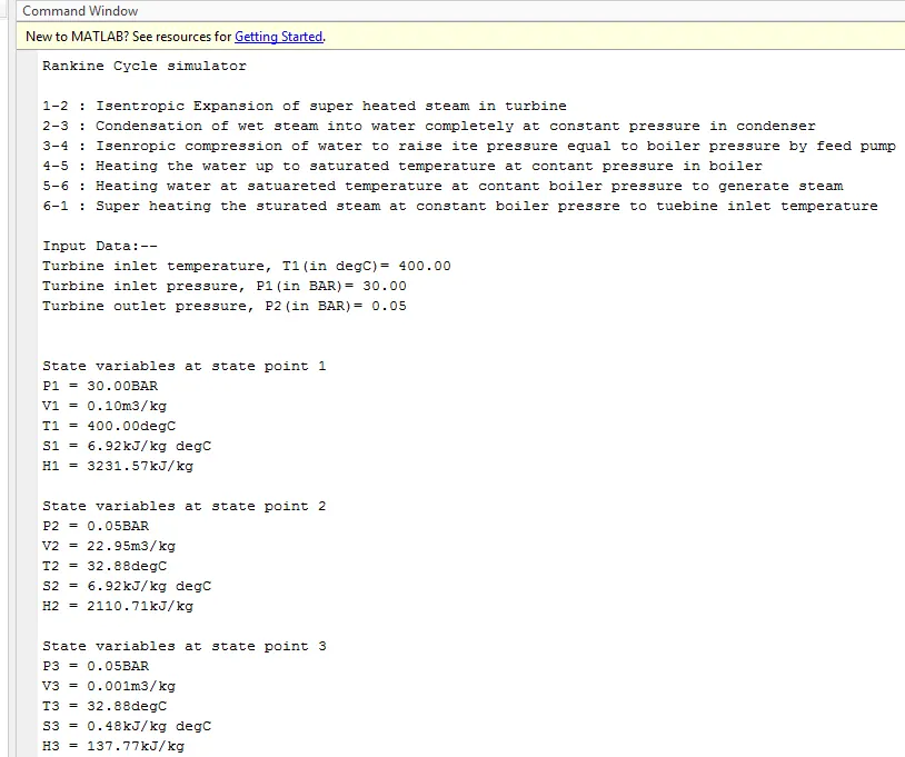
In th code , first the input datas are taken. These are Turbine inlet pressure P1=30bar, Turbine inlet temperature T1= 400degC, Turbine outlet pressure P2=0.05Bar.
After that state varriables for 6 state points, are calculated. For this the XSteam library is downloaded from the link given to get steam table data.
For the state point-1, T1, P1 are already given, value of V1(specific volume in m3/kg), H1(specific enthalpy in kJ/kg), S1(specific entropy in kJ/kg degC) are obtained from using XSteam library downloaded. Here we see the steam feede in to tubine (or obtainned from boiler) is superheated steam.
Process 1-2 is isentropic expansion of steam in turbine. After expansion the steam becomes wet. Here entropy remains constant. S2=S1.
So for the state point 2, the dryness fraction(x) of the steam is calculated. With the vlaue of 'x' & by using XSteam library we get the values of S2, H2 , V2 & T2 calculated. P2 is given as input data.
Besides this, to get inbetween points of 1-2 process,the formula ( p*v^n=constant) is used. Here value of 'n' is calculated & from that, value of constant is evaluated. Hence the values of inbetween points of 1-2 process have been defined.
Process 2-3, is a constant pressure & temperature process . Here wet steam from turbine is condensed in condenser into water completely. So for the state points 2 & 3, there are no change in pressure & temperature. So P2=P3 & T2=T3. Accordingly S3,H3 are calculated & V3 is obtained from XSteam library.
The process 3-4 is isentropic compression of saturated water by feed pump. So here entropy remains constant(S3=S4). In this perocess the pressure of water is raised to boiler pressure. So P4=P1 (P1 is boiler pressure). Here work is done by feed pump on the water. Work done by feed pump is calculated, which is used to find out the enthalpy at state point 4 (H4=H3+Wp). Cp4 & Cv4(Specific heat of water at constant pressure & constant volume for state point 4) are calculated by using XSteam library. Cp4,Cv4 & the formula (T^k*P^(k-1)=constant , where k=Cp4/Cv4) are used to find the value of T4 . V4 is calculated from XSteam library.
The process 4-5 is heating of water in boiler at constant boiler pressure (P4=P5=P1) & at the end of the process(at state point 5) it will be stuarated water at pressure P1. The satutation teperature at pressure P1 is T5. For the state point 5, the values of V5, T5, H5, S5 are calculated using XSteam library
The process 5-6 is the process of generating saturated dry steam. So heat given, is the latant heat to produce the dry stuarated steam. So here pressure & temperature remain constant. So P6=P5=P1(=boiler pressure=40Bar) , T6=T5. For the stae point-6, V6, S6, H6 are calculated by using XSteam library.
The process 6-1 is superheating the dry staurated steam at constant boiler pressre, to raise the temperaure of steam to T1(Turbine inlet temperature=400degC which is one of the input data for this program). Here pressure remains constant so P6=P1(which is also turbine inlet pressure).
Now after getting all the state varriables, Work done by Turbine(W_t), Work done by feed pum (Wp), Net work done (W_net), Back work ratio(BWR), Specific steam consumption(S.S.C) are calculated.
After this data to plot liquid line & dry saturated staem line are calulated. The critical temperature 374.15degC is used here. At this critical point the latent heat of vaporization is zero & at this point liquid & vapour phases merge & become identical in every respect. The corresponding pressure at this point is 221.2Bar.
For getting points of liquid line & dry satuarated line in T-S & H-S diagram, a for loop & XSteam library are used.
Plotting P-V diagram:--
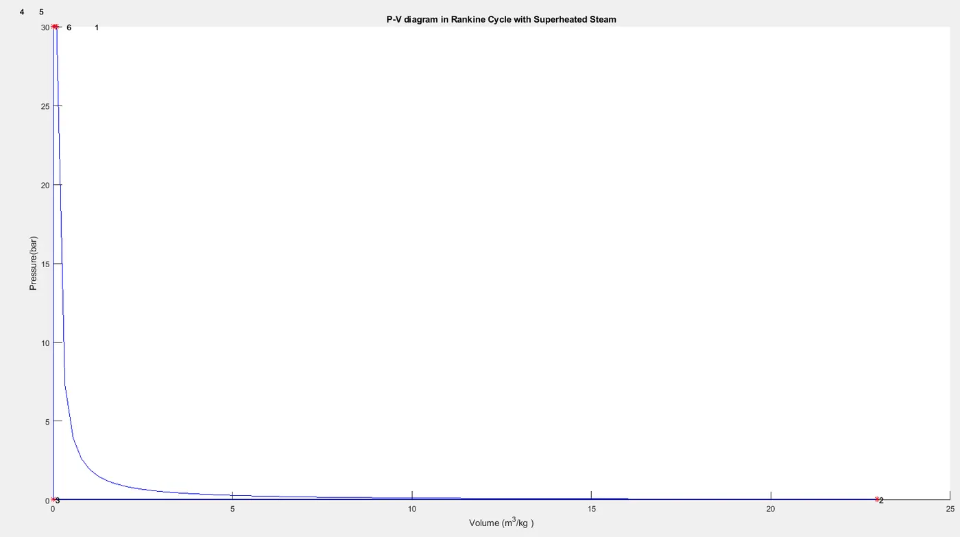
Code for plotting of P-V diagram is written. Figure 1 is created for P-V diagram. In this plot the isentropic expansion of steam is shown by 1-2 curve. Other process are represnted by straight lines.The P-V diagram is given below
Plotting T-S diagram:--
For plotting T-S diagram, Figure 2 is used. The T-S diagram is given below.
In this diagram, the blue line represnts the T-S plot. The red line represents the sturated liquid line & dry stuarated steam line.
In the plot, the process isentropic expansion of steam in turbine & isentropic compression of water by feed pump are represented by straight lines 1-2 & 3-4 respectively. Here as entropy is constant, the representing lines are vertical straight lines.The straight line 2-3 represents condensation of steam at constant temperature. The straight line 4-5 represents the heating of water to saturated temperature in boiler. The straight 5-6 represents ths the process of generating dry sturated steam at constant temperature in boiler. The curve 6-1 represents the super heating of steam at constant pressure in boiler. For getting the curve 6-1, a for loop & XSteam library are used. s61, & t61 are the inbetween points of the curves 6-1.
Plotting S-H diagram:--
For this diagram Figure-3 is used.The diagram is given below.
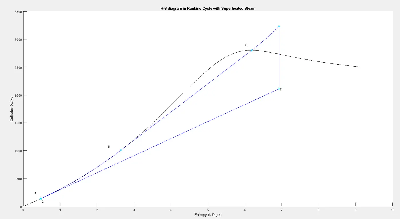
The blue lines represent the S-H plot, & black lines represent the liquid line & steam line.
The straight lines 1-2 & 3-4 represent the two isentropic process. For other process (2-3, 4-5, 5-6 & 6-1) the curves are obtained by using 'for loops' & XSteam library.
After this, code for creating display of Heading, The processes, The stae varriables, Work done by Turbine, Pump workdone, Back work ratio, Rankin cycle efficiency, Specific steam consumption at the command window, are written.
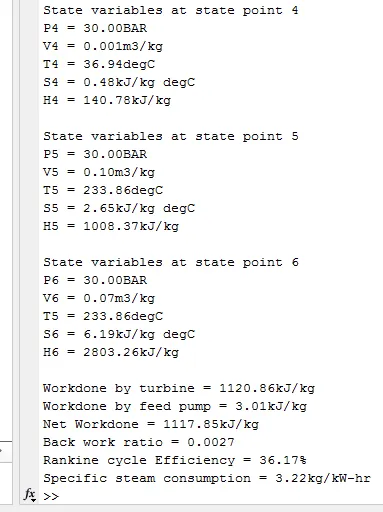
The screen shots of the displays are given below.