Week 3 - Solving second order ODEs

AIM: Your objective is to write a program that solves the following ODE. This ODE represents the equation of motion of a simple pendulum with damping.

Theory:

The presented project report attempts to provide a comprehensive study and develop a script for solving second order differential equations for the transient motion using MATLAB. MATLAB is software featuring a high-level programming language, primarily intended for numerical computations. Octave helps in solving linear and nonlinear problems numerically, and for performing other numerical experiments to describe the transient behaviour of a system.

A simple example is a pendulum. The way the pendulum moves depends on Newton's second law. When this law is written down, we get a second order Ordinary Differential Equation that describes the position of the "ball" w.r.t time.

An ordinary differential equation (ODE) is a differential equation containing one or more functions of one independent variable and the derivatives of those functions. The ODE equation and the calculations are shown below:

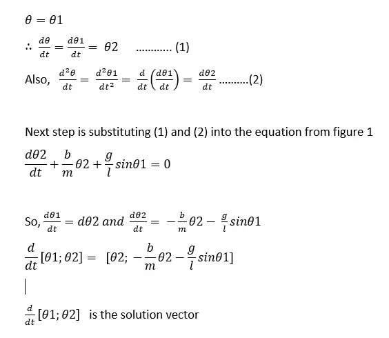
The simple pendulum consists of a point mass m hanging on a string of length L from some support. One pulls the mass back to some starting angle, θ0, and releases it. The goal is to find the angular position as a function of time.

We could either use Newton’s Second Law of Motion, F = ma, or its rotational analogue in terms of torque, τ = Iα. We will use the former only to limit the amount of physics background needed. There are two forces acting on the point mass. The first is gravity. This points downward and has a magnitude of mg, where g is the standard symbol for the acceleration due to gravity. The other force is the tension in the string. In these forces and their sum are shown. The magnitude of the sum is easily found as F = mg sin θ using the addition of these two vectors.

Now, Newton’s Second Law of Motion tells us that the net force is the mass times the acceleration. So, we can write mx¨ = −mg sin θ. Next, we need to relate x and θ. x is the distance travelled, which is the length of the arc traced out by the point mass.

This ODE represents the equation of motion of a simple pendulum with damping.

Given Parameters:

g (m/s2)	gravity	9.81 m/s2
m (kg)	mass of the ball	1 kg
b	damping coefficient	0.05
L (meter)	The length of the pendulum	1 meter
Time Interval	Simulation motion	0-20 sec

angular displacement=0,

angular velocity=3 rad/sec at time t=0.

The Function code is shown below:

 function[dtheta_dt] = ode_func(t,theta,b,g,l,m)
  
 theta1 = theta(1)
 theta2 = theta(2)
 dtheta1_dt = theta2;
 dtheta2_dt = -(b/m)*theta2-(g/l)*sin(theta1);
 dtheta_dt = [dtheta1_dt;dtheta2_dt];
 
end

A function is a group of statements that together perform a task. In MATLAB, functions are defined in separate files. The name of the file and of the function should be the same. Functions operate on variables within their own workspace, which is also called the local workspace, separate from the workspace you access at the MATLAB command prompt which is called the base workspace.

Function handles are simple to function codes that can be created without using the regular function definition using the keywords ‘function’ and ‘end’. They do not require any separate ‘.m’ files or not needed to be declared separately below/above the main code. Function handles are directly declared in the main code itself and also accessible from any point in that particular code, i.e they are localized to a particular conditional. The declaration of a function handle is very similar to that of a function declaration. It can be distinguished by the means of the ‘@’ symbol before your value/expression allocation. The syntax for creating a function handle is. A function was defined in order to establish a relation between all the given input values, the function code is based on the equation derived in the above equation figure.

Main code of the Project:

% write a program that solves the following ODE. This ODE represents the equation of motion of a simple pendulum with damping.

close all 
clear all 
clc

% Input data
L=1;             % length of the pendulum in m,
m=1;             % mass of the ball in kg,
b=0.05;          % damping coefficient.
g=9.81;          % gravity in m/s2,

% Initial Condition

theta_0 = [0;3];   % we have 2 first order diffrencial equations , one id for displacement and other one is for velocity
    % So here initial displacement is 0 and initial velocity is 3 m/s
    
% time between 0-20 sec,
t_span = linspace(0,20,250);

% Calling function in side ode45 for diffrent values of time t_span and intial condition 
%@(t, theta) meant ode_func is the  function of t and theta,
% ode_func(t, theta,b,g,L,m) is how Ode is defining
% t_span how much time we have read reasults
% theta_0 is reads the vaules of displacement and angular velocity for every value of t_span
% we will get angular velocity, displacement at time 't'

[t,results] = ode45(@(t,theta) ode_func(t,theta,b,g,L,m),t_span, theta_0);

% Plots
figure(1)
plot(t,results(:,1),'linewidth',1.5)
hold on
plot(t,results(:,2),'linewidth',1.5)
grid on
xlabel('time in s')
ylabel('angular displacement in theta and Velocity in m/s')
legend('angular displacement',' Velocity')


%  pendulum animation
ct = 1;
for i = 1 : length(results(:,1)); % where i value varies from 1 to length of results in first column i e angular displacement
 % consider for fixed end of pendulum is at x0 and y0
 x0 = 0;
 y0 = 0;
 
 % for the coordinates x1 and y1, which are varing wrt angular displacement,
 % x1 = length of string * sind(theta) and  y1 = length of string * cosd(theta)
 
 x1 = L*sin(results(i,1));       % coordinate value at theta1 in x axis      
 y1 = -(L*cos(results(i,1)));      % coordinate value at theta1 in y axis 
 
 % plots
 figure(3)
 plot([-5 5],[0 0],'color','k' ,'linewidth',5 );
 axis([-2 2 -1.5 0.5])
 hold on
 plot([x0,x1],[y0,y1],'linewidth',3,'color','b');
 plot(x1,y1,'o','markersize', 20, 'markerfacecolor', 'r','color','b');
 pause(0.03)
 hold off

%Create Gif
printf('Creating GIF- Progress... %d', ct)
ct = ct + 1;
img = print ('-RGBImage'); 
imwrite(img, 'animation.gif', 'DelayTime', .005, 'Compression', 'bzip', 'WriteMode', 'Append'); 
 
end

Before writing the code, it's important to start with clear all, close all and clc commands since

Clear all - removes data from the workspace, freeing up system memory

Close all- deletes the current figure or the specified figure

clc - clears all input and output from the Command Window display, giving you a "clean screen

The next step is to define the inputs and variables. The damping coefficient, gravity, length of the spring and mass of the bob have all been defined.

The next step is to define the initial conditions, the angular displacement and angular velocity have been defined. Timespan has also been defined.

The next step is to solve the ODE, Ode45 was used, it is a function in Matlab that solves ordinary or partial differential equations using a numerical method. The numerical method in question here is the 4th order Runge Kutta method. The function ode45 takes 3 inputs. The 3 inputs are the function to be integrated, the time span and the initial conditions. [t, results] means that the results have been calculated with respect to time.

Creating GIF

• Line 1: printf('Creating GIF- Progress... %d/%dn', i, length(t_span));

This statement helps us keep track of the GIF creation progress. As mentioned earlier Octave is not that efficient and this process can take a bit of time. Therefore, it is important to keep track of the progress so that one can have a rough estimate of the completion time.

printf - This function is used to print a particular string in the command window. The string we want to print is ‘Creating GIF- Progress... %d/%dn’.

%d - This is a format specifier. This tells the printf command that a number (integer) should come in this place. The number is mentioned later.

n - This character creates a new line every time it gets executed. We don’t want to print the progress all in one line.

i - This is the loop variable. The value of this variable is incremented by 1 at each new for loop iteration.

t_span - This is the marching-step array. A new plot is obtained for each value of t_span and we need to stitch these into an animation.

length() - This function returns the total number of elements inside an array.

After calculating the results, a graph has to be plotted, the graph contained two plots. One for angular displacement with respect to time and one for angular velocity with respect for time.

• Line 2: img = print ('-RGBImage');

We need to create an image object before starting to write it into a gif file. This statement helps us achieve that. It fetches the current plot image and stores it inside the mentioned variable.

print() -. The “print” command saves the most recent plot that has been generated. Here we don't need to save the image physically. So we are storing the image inside the variable ‘img’. In general, Octave supports four different kinds of images, grayscale images, RGB images, binary images, and indexed images. Here, we’re using the RGB format.

-RGBImage - This option returns the plot image in the RGB format. The image is represented by a matrix M by N by 3 where each of the 3-vectors corresponds to the red, green, and blue intensities of each pixel.

• Line 3: imwrite(img, 'animation.gif', 'DelayTime', .005, 'Compression', 'bzip', 'WriteMode', 'Append');

This statement creates an animation file and keeps attaching the current plot image at each iteration. It also specifies the display time for each image frame inside the gif file and also asks the octave to compress each image before appending it into the gif file.

imwrite() - This function is used to write images in various file formats.

img - The image to be written into the gif file is stored inside img.

animation.gif - This is the name of the output gif file. From the name itself, Octave can figure out that the output is going to be a gif file.

DelayTime - This property is used to specify the delay between each frame (image) i.e., at what speed the gif should be displayed. It controls how long a frame is displayed until it moves to the next one. The value for the property should be in seconds. Here we have provided the delay as 0.005 seconds.

Compression - The raw images obtained using the print function are large in size. So we need to compress to bring each image into a minimum size as it's attached to the gif file. This property is used to accomplish that. The type of compression is mentioned as the value for this property. Here, we’re using the ‘bzip’ compression.

Output:

1. The output obtained is a graphical representation of the velocity curve and displacement curve w.r.t Time.

• Angular Displacement and Angular Velocity plots were generated for a time range of 20 secs.

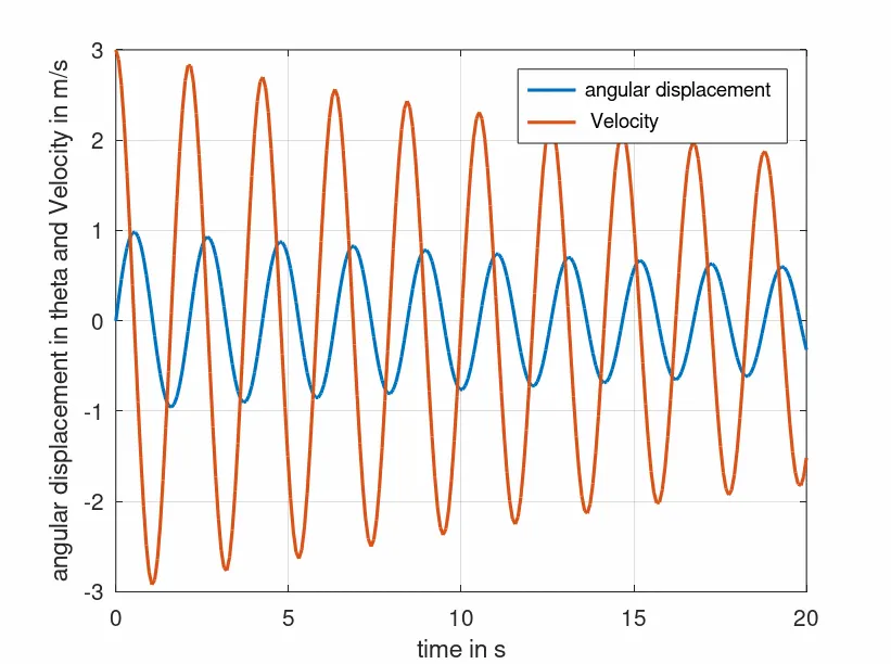
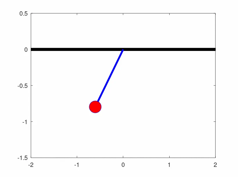
Finally, on executing the code, each new image corresponding to a new for loop iteration is attached & created into an animation in GIF format. The resulting GIF format looks like given below:

Conclusion:

The simulation of the transient behaviour of a simple pendulum is successfully created by using a program in MATLAB.