Week 3 - Solving second order ODEs

Objective:

Create a Matlab Program to solve an ODE of equation of motion of Simple Pendulum with damping and create an animation simulating the motion of the Pendulum.

Theory and Methodology:

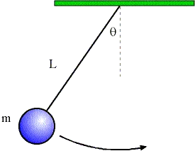
The equation of motion of Simple Pendulum with Damping is as follows

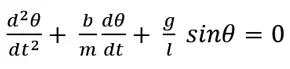………….. (1)

Where ,

Angular Displacement of Pendulum.

t=Time

g = gravity in m/s2,

l = length of the pendulum in m,

m = mass of the ball in kg,

b=damping coefficient.

Let,

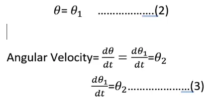
Thus, the eqn (1) can be modified as,

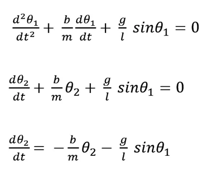
Thus, we have converted the Second Order Differential equation into two First Order Differential Equations. This two equations can be written in Matrix form and used to solve the differential equation.

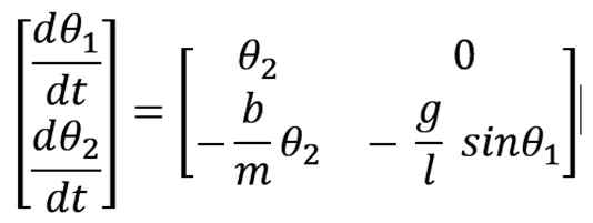
Now, we will draft this equation in Matlab as a function we can call for specified values t,theta,b,g,l,m .

Code for ode_func Function:

function [dtheta_dt]=ode_func(t,theta,b,g,l,m)

theta1=theta(1);
theta2=theta(2);
dtheta1_dt=theta2;
dtheta2_dt=-(b/m)*theta2-(g/l)*sin(theta1);
dtheta_dt=[dtheta1_dt;dtheta2_dt];
end

Now, We will code the Program to :

1)Solve the Motion Equation of the simple pendulum with damping(Second order ODE)

2) Calculate position of Pendulum for different values of time,

3) Then Simulate the Motion of the Simple Pendulum and make a movie of the animation.

We will start the program with clearing the temporary memory and the command window and closing all outputs.

We will input the specifications of the Simple Pendulum and the initial values of Angular velocity and Angular Displacement.

Then we will create an array for different time values at which the motion is to be simulated.

Then to solve the two first order differential equations as embedded in the ode_func we will be using the in-built ode45 function of MATLAB.

ode45 is a versatile ODE solver

ode45 syntax:

[t,y] = ode45(odefun,tspan,y0)

where tspan = [t0 tf], integrates the system of differential equations y′=f(t,y) from t0 to tf with initial conditions y0. Each row in the solution array y corresponds to a value returned in column vector t.

odefun is the differential function that needs to be solved for initial value y0 and through time_span.The function returns values of y at different t.

We can code accordingly.

[t,results]=ode45(@(t,theta)ode_func(t,theta,b,g,l,m),t_span,theta_0);

Here the output is stored in variables results and t. Results stores the values of Theta1 and Theta2 i.e Angular Displacement and Angular Velocity calculated at each time step. T stores the values of each time-step.

Then we can plot the Angular Displacement as stored in results array at 1 and Angular Velocity as stored in results array at 2.

Then to simulate the motion of Pendulum. We will plot the position of Pendulum for every time step. We will use for loop for number of iterations as the number of time-steps and the number of different positions of pendulum for calculated every Angular Displacement.

One end of the string will be fixed (0,0)and the other end will be position of Ball or Bob can be calculated from Angular Displacement by getting x and y coordinates for l.sin and l.cos respectively.

Then we will plot the Ball as a marker. This will be a single frame for any instance of time step. All such instances will be saved in a variable. Thus, for every iteration of for loop a frame will be created and stored.

Later we will compile all the frames and animate the motion of the pendulum and save the movie.

Code:

clear all
close all 
clc

%Parameters of System
b=0.05; %Damping Coefficient of system
g=9.81;  %Accceleration due to gravity  
l=1;  %Length of the String
m=1;  %Mass of the Bob

%INITAL CONDTIONS
theta_0=[0;3];   % Values of Angular Displacement and Angular Velocity at t=0 sec

%Time points
t_span=linspace(0,20,500);  % Time Period of 20 secs from t0 sec with 500 time steps 

%Solve ODE
[t,results]=ode45(@(t,theta) ode_func(t,theta,b,g,l,m),t_span,theta_0);

%Plot Angular Displacement and Angular Velocity 
figure(1)
plot(t,results(:,1))
hold on
plot(t,results(:,2))
ylabel('Plot')
xlabel('Time')
title('Second Order ODE')
legend('Angular Displacement','Angular Velocity')
hold off

% Plot the Position of Pendulum for each time step
ang_disp=results(:,1);
ct=1;
figure(2)
for i=1:length(ang_disp)
    
    T=ang_disp(i);
    % Fix end of the string
    x0=0; 
    y0=0;
    %Position of the ball or bob
    x1=l.*sin(T);
    y1=-l.*cos(T);
    
    %Plot Fixed support
    plot([-0.5 0.5],[0 0],'linewidth',3,'color','black')
    hold on
    %Plot the string as line
    plot([x0 x1],[y0 y1],'linewidth',1,'color','b')
    hold on
    %Plot the ball/bob as a marker
    plot(x1,y1,'bo','MarkerSize',20,'MarkerEdgeColor','red','MarkerFaceColor','red')
    hold on
    %Plot the hatchings of fixed support
    plot([-0.5 -0.4],[0 0.1],'linewidth',1,'color','black')
    hold on
    plot([-0.3 -0.2],[0 0.1],'linewidth',1,'color','black')
    hold on
    plot([-0.1 0],[0 0.1],'linewidth',1,'color','black')
    hold on
    plot([0.1 0.2],[0 0.1],'linewidth',1,'color','black')
    hold on
    plot([0.3 0.4],[0 0.1],'linewidth',1,'color','black')
    hold on
    plot([0.5 0.6],[0 0.1],'linewidth',1,'color','black')
    hold off
    %Set Axes of Plot
    axis([-1 1 -1.5 0.5])
    pause(0.05)
    title('Animation of Damped Oscillations of a Simple Pendulum')
    legend('Fixed Support','String','Mass/Ball')
    M(ct)=getframe(gcf); %Store this plot as a frame in a variable
    ct=ct+1;
end

% Compile all the frames to create a movie and save it
movie(M)
videofile=VideoWriter('Simple_Pendulum.avi')
open(videofile)
writeVideo(videofile,M)
close(videofile)

Errors Faced:

1)

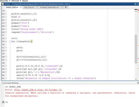
The syntax error for for loop statement because of wrong use of semi-colon which was removed.

2)

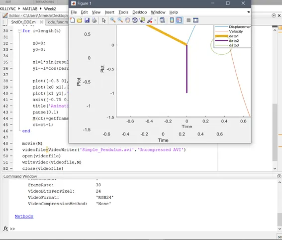
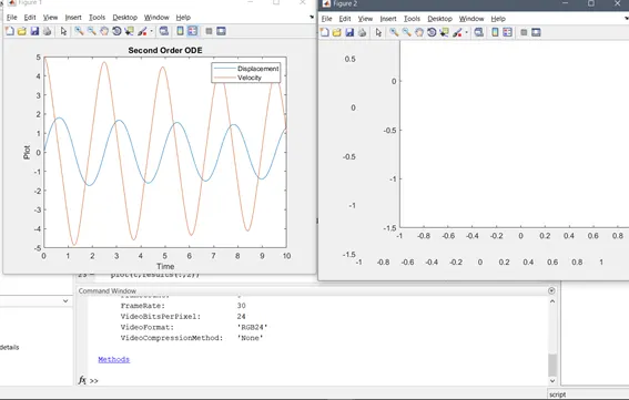
The Plot was not generated properly because of improper use of hold on function and wrong declarations in plot command. It was all corrected.

Output:

1)Plot of Angular Displacement and Angular Velocity with respect to Time.

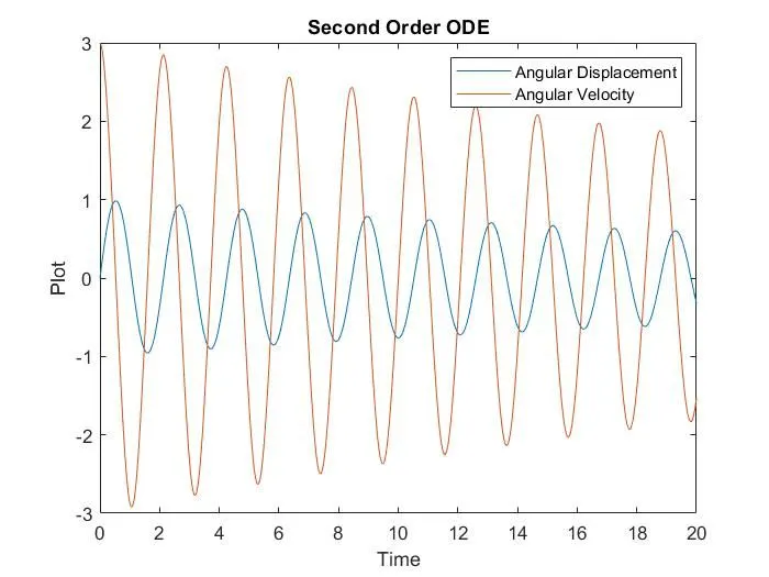
At the start point,at t=0 Angular displacement is 0 at the extreme topmost point.Then with time the displacement starts icreasing till it is maximum at the bottommost point and then starts decreasing till 0 at the other topmost point and then decreases further for crest value.Then once it reaches crest it again starts increasing through 0 till the peak value.

However, the angular velocity at the start at topmost is the maximum peak value which then approaches 0 value at bottommost point and further reduces to Crest value at opposite topmost point.Then again it starts increasing through 0 till the peak value and this goes on.

The oscillating motion can be observed from the plot. As the system is damped we can see the amplitude decreasing over time.

2) Animation of Simulation of Motion of Simple Pendulum with Damping:

The above video depicts the simulation of motion of the Simple Pendulum with damping. We can see the pendulum oscillating from extreme righttop position to extreme lefttop position with recurring over spans of time. And over the time we can observe the amplitude of Pendulum reducing due to damping.