Flow over a cylinder

Aim:
1) Run a Baseline simulation and calculate Reynolds number.
2) Run transient flow simulations for each case of increase in Reynolds number by factore of 20%, 40% and 100% .
3) Create Animations for Pressure Velocity for all the cases.

Theory:

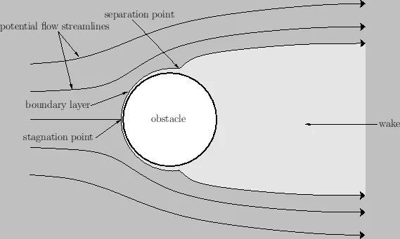
Boundary Layer Separation:
For a external flow over a body, the detachment of a boundary layer from the surface of body is known as Boundary layer separation. Boundary layer may be laminar, transition or turbulent and its thickness goes on increasing in direction of flow. Pressure goes on decreasing till the half of the body and then starts to increase in other half. Thus fluid experiences an adverse Pressure gradient .Thus flow separates from the surface .
Separation Point: The point on the profile at which the boundary layer seperates is Seperation Point.At this point velocity is maximum.
Stagnation Point: The point on body at which the fluids comes to rest i.e velocity is zero or minimum and pressure acting is maximum is stagnation point.
Wake : Due to adverse pressure effect the fluid has to move against the increasing pressure which causes fluid to stop or get reversed. This results in area of reverse flow creating highly turbulent region behind the body called as Wake region.This causes Aerodynamic Drag.
Vortex Shedding:The boundary layer seperates from the surface and forms a shear layer which is highly unstable. This layer rolls into a discrete vortex and detaches from surface and this phenomenon called as Vortex Shedding. These vortices are shed alternately from top and bottom surface which form the Vortex Street. This occurs at Discrete Frequency given by
Strouhal Number: St=fD/v
where St=0.21 for Re greater than 1000.

Methodology:
For a Baseline case,
diameter of cylinder,d=0.05m
Length of cylinder, L=0.05m
Velocity, v=1 m/s
For Air as fluid,
Density, =1.225 kg/m³
Dynamic Viscosity, =18.6×10^-6 uPa.s

Re= (1.225 x 1 x 0.05)/18.6×10^-6
Re=3293.01

Flow through Time, FTT=DOMAIN LENGTH(X)/Velocity

End Time = ET=2FTT.

Time Step = ET/10 ....for 10 steps.

Now lets calculate Reynolds number and Velocities for increase in baseline Re by 20%,40%and 100% respectively.
1) 20 % rise
Re=Re+20%Re
=3293.01 + 0.2(3293.01)
=3293.01 + 658.602
=3951.612

Now, v=Re.μ/ρ.d

v=(3951.612 × 18.6 ×10^-6) /(1.225×0.05)
v=1.2 m/s


2)40% rise
Re=4610.214
v=1.4 m/s

3) 100% rise
Re=6586.02
v=2 m/s


Now we will model a cylinder of mentioned dimensions in the Solidworks modeller and save the Part.

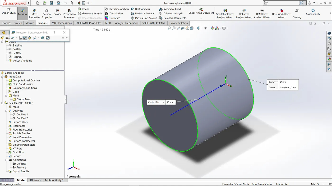
Then we will setup a Flow Simulation using the wizard to choose a suitable computational domain.
For default
+x =0.3 m
-x= -0.2 m
Thus total Domain length is 0.5 m

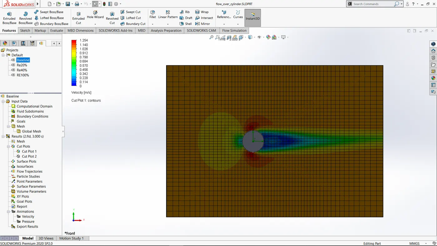
But this is inadequate as seen. Thus changing the domain size along X axis.

For +x =0.6 m
-x= -0.4 m

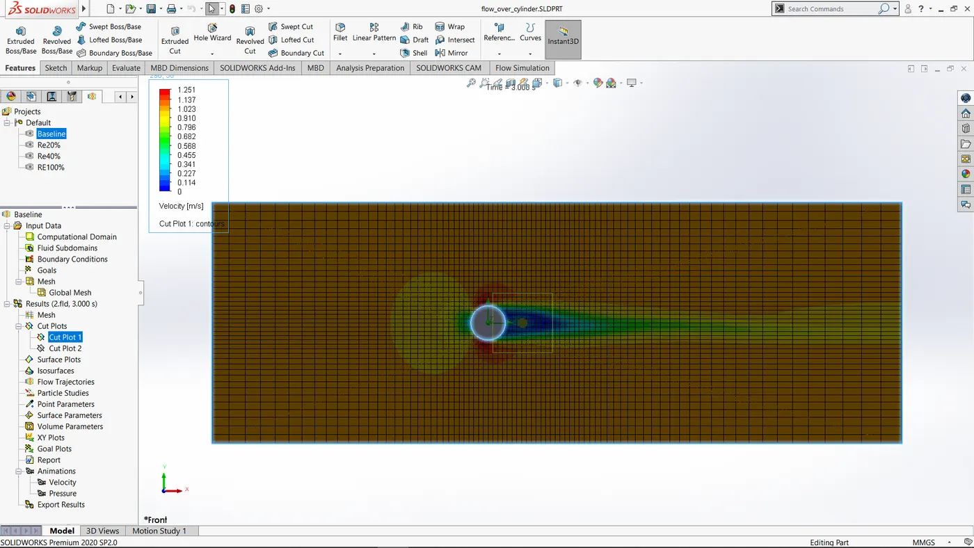
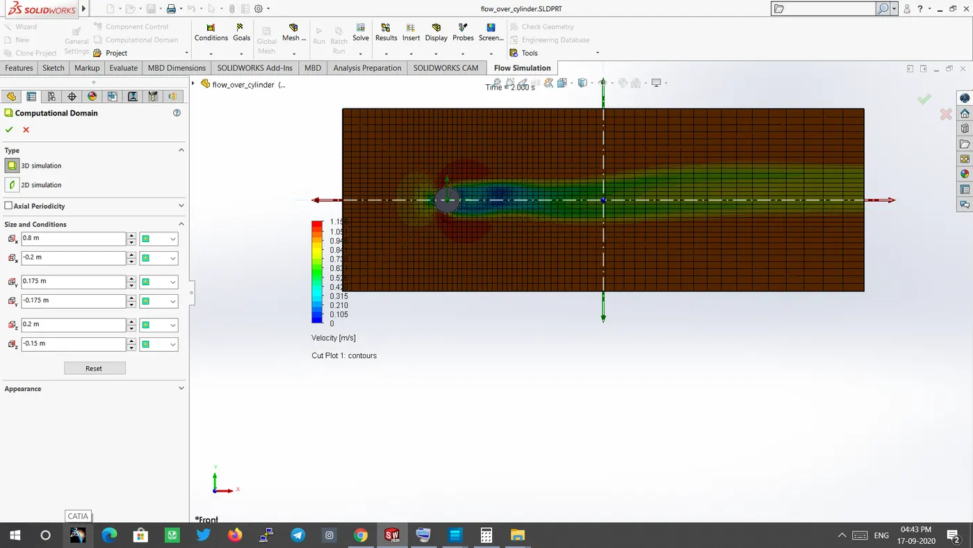
Now we have chose domain length
+x = 0.8 m
-x = -0.2m
Thus total Domain length is 1m.

Thus now we can calculate FTT and ET.

1) For Baseline Case
FTT= 1/1
=1 sec
ET= 2FTT
= 2 sec
Step= ET/10
=0.2

2) For Re20%
FTT=0.833 sec
ET=1.66 sec
Step=0.166

3) For Re40%
FTT=0.71 sec
ET= 1.42 sec
Step= 0.142

4) For Re100%
FTT=0.5 sec
ET= 1 sec
Step = 0.1

Now we will setup flow simulation for Baseline case.

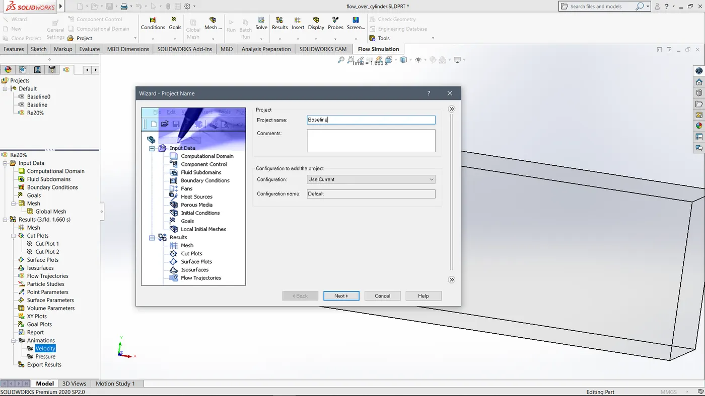
Choose External flow and input ET in Total Analysis time and Step in Output time step.

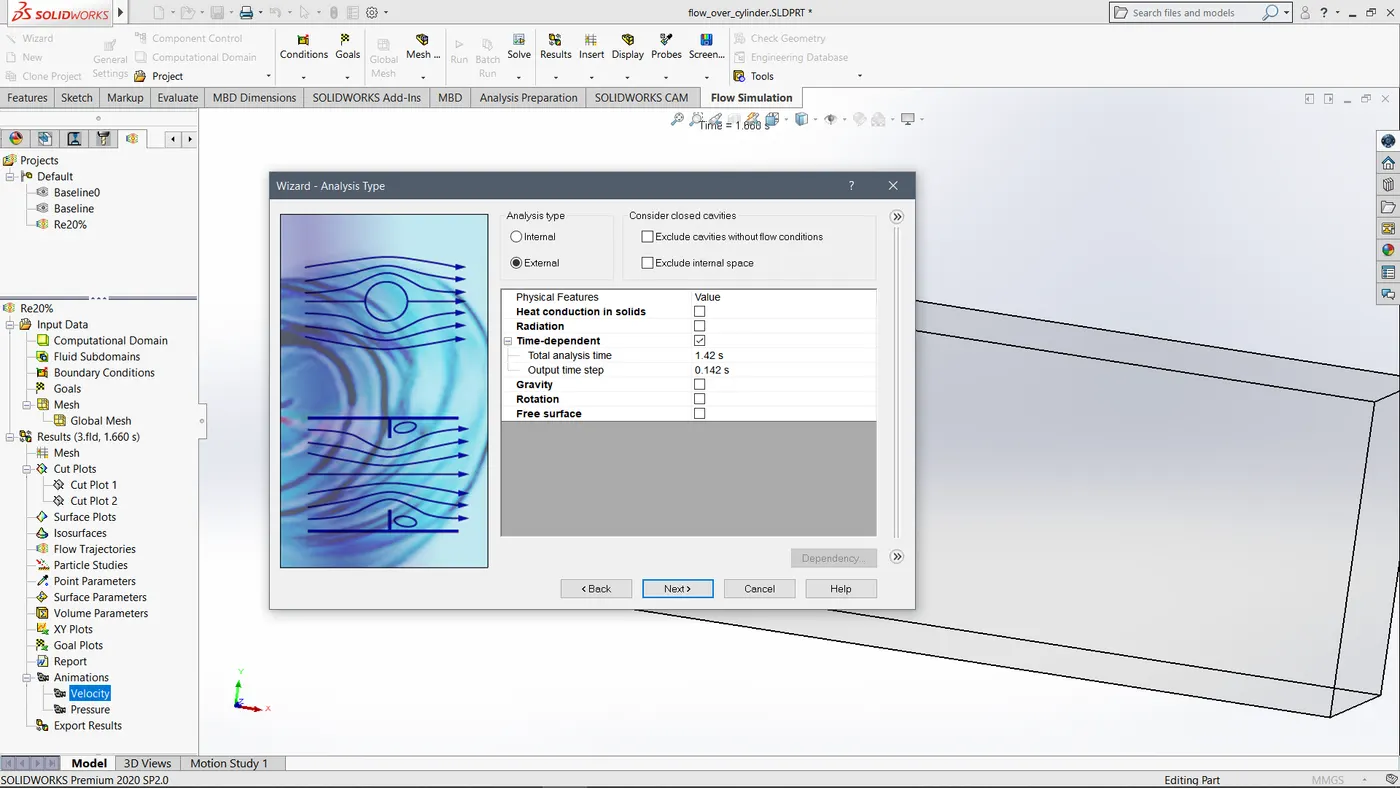
Then selecting air as fluid.And inputing velocity along X as 1 m/s.

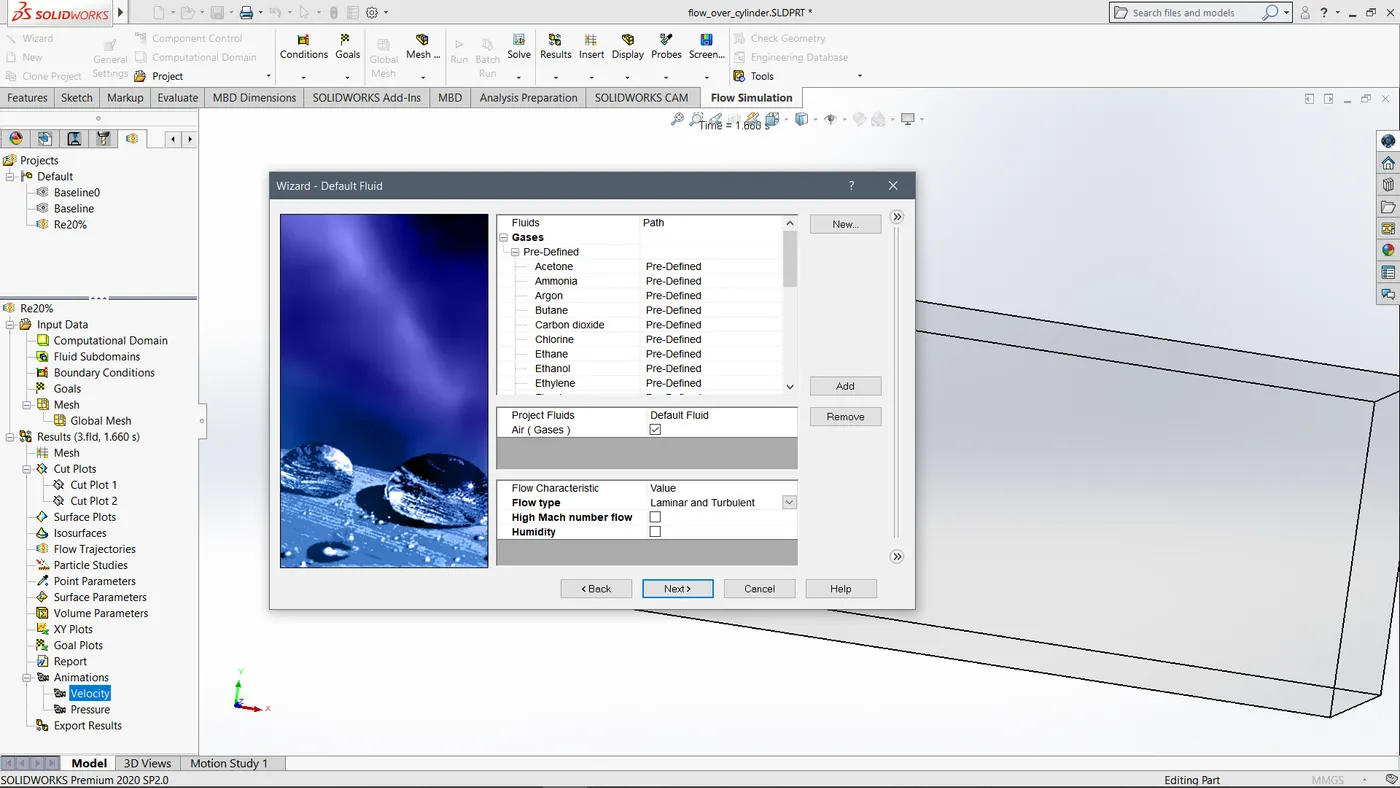
Then we will setup the Computational Domain to proper size and adjust mesh as per need.
Then in Results we will add Cut Plots for Velocity and Pressure and then Run the simulation.

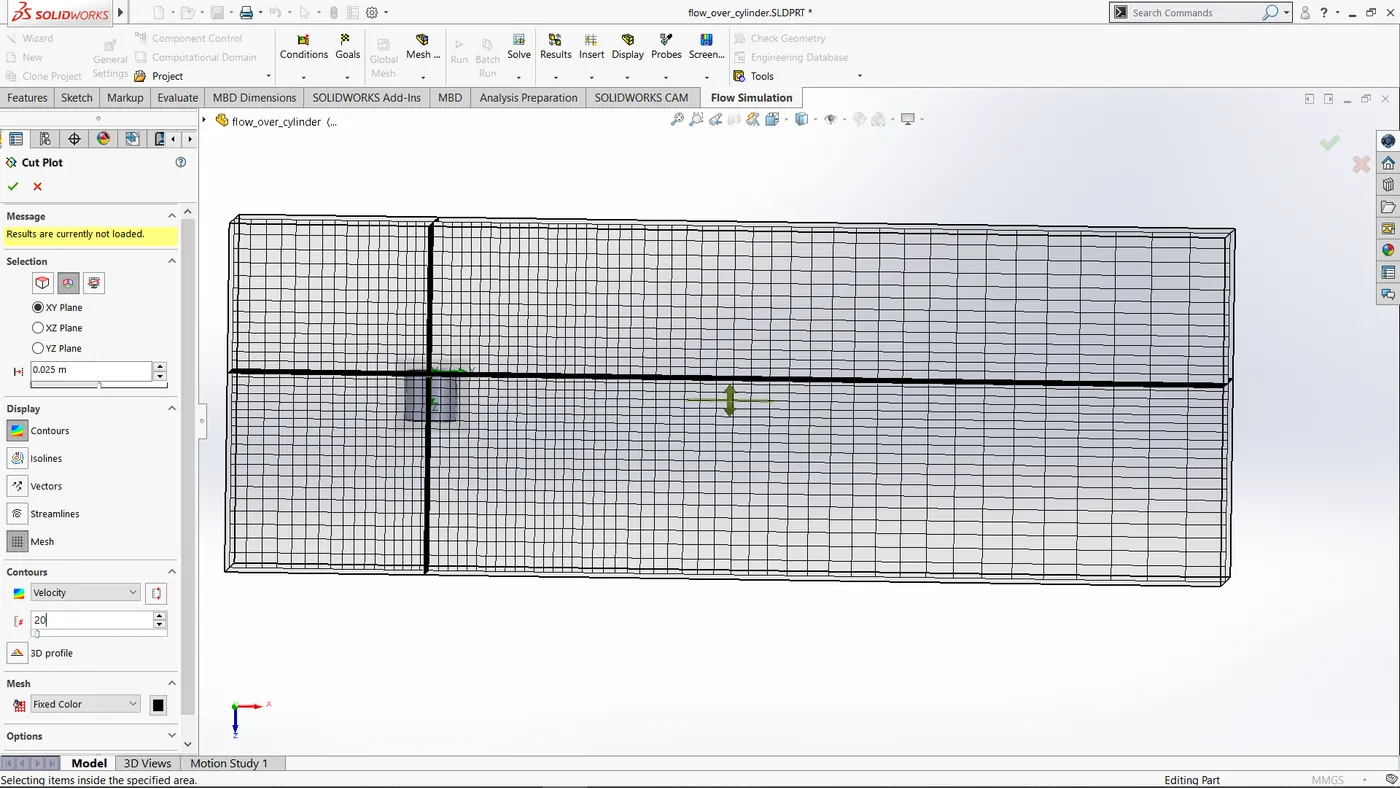
Once the simulation is complete we will insert Animation for Velocity and Pressure by selecting Delete previous animations and selecting Scenario for Transient animation and animation for 10 secs.

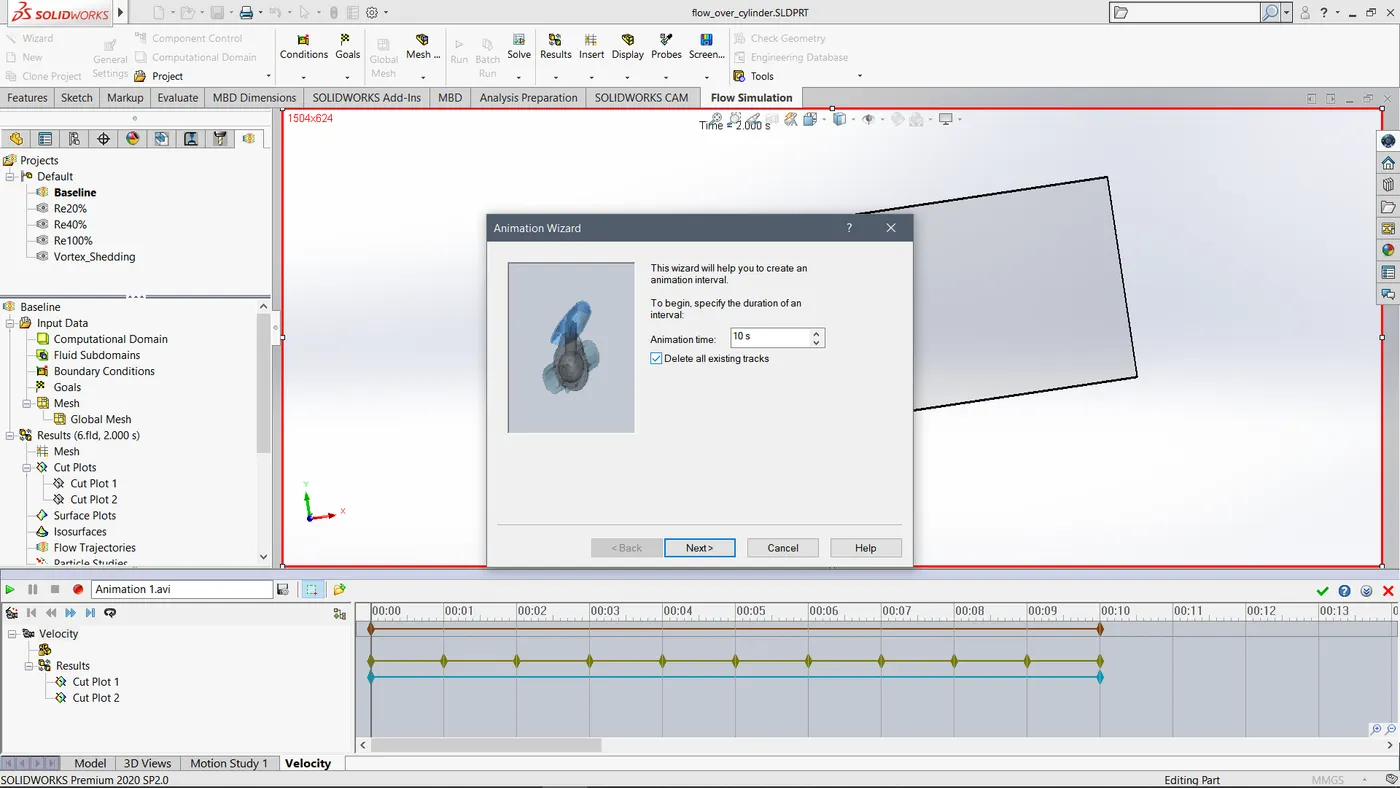
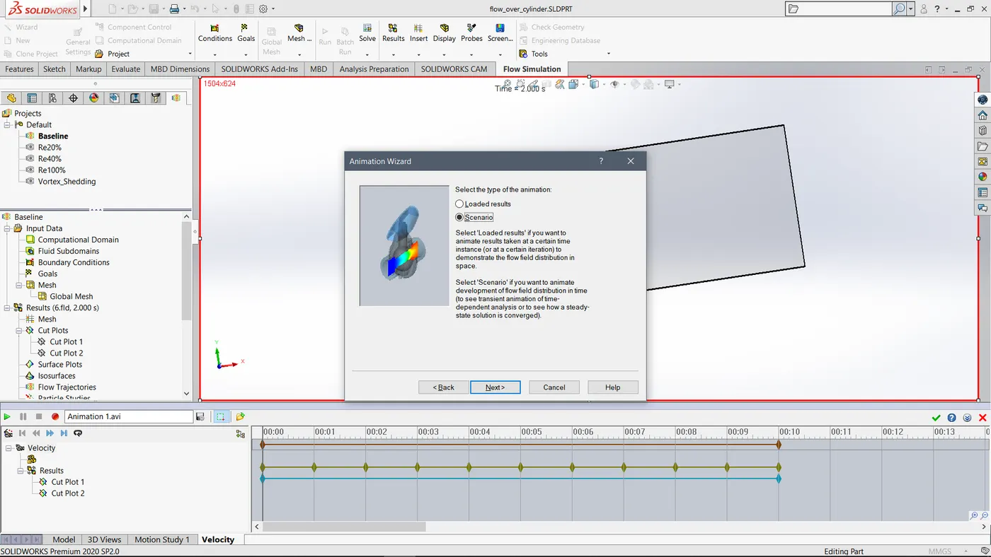
Similarly we will setup Flow Simulation for all other cases and create Cut Plots and animations.

Results and Observations:

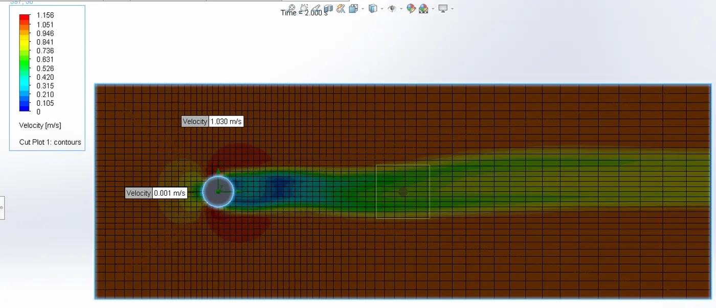
1)Baseline :
Velocity Plot

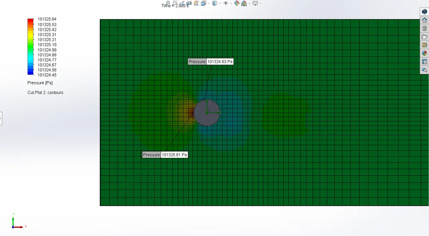
Pressure Plot

Velocity animation

Pressure animation

2)Re20% :
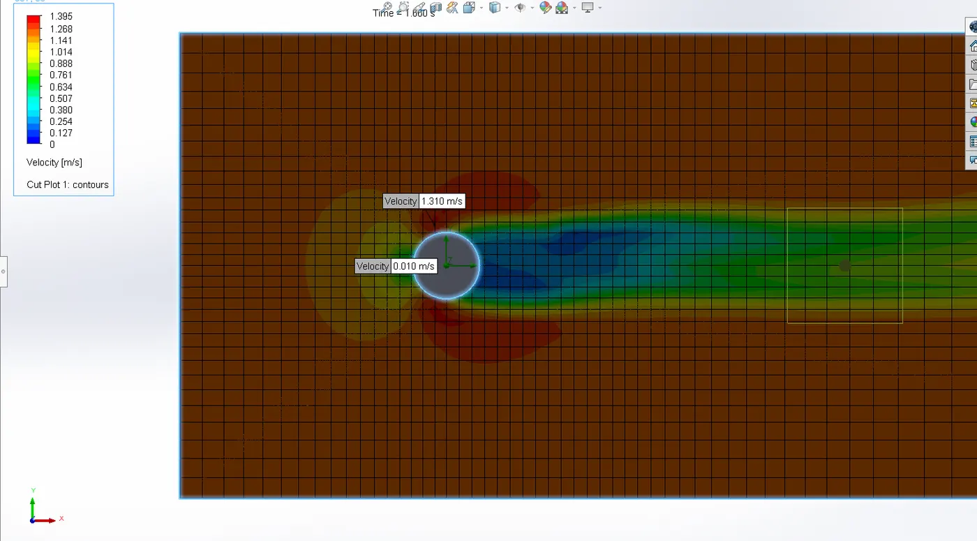
Velocity Plot

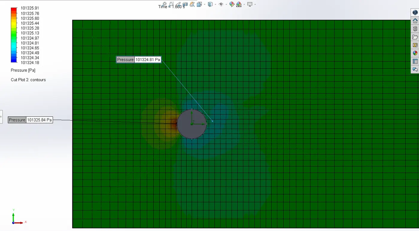
Pressure Plot

Velocity animation

Pressure animation

3)Re40% :
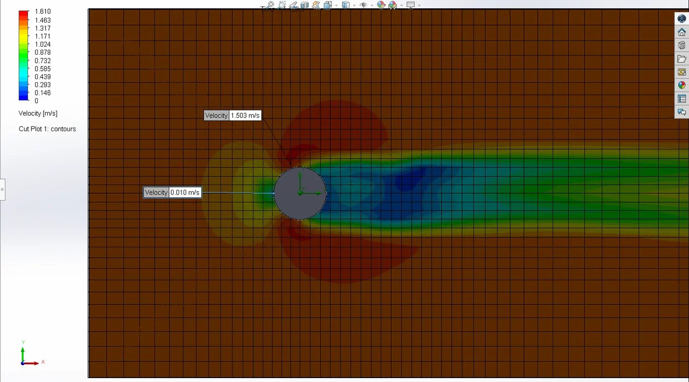
Velocity Plot

Pressure Plot

Velocity animation

Pressure animation

4)Re100% :
Velocity Plot

Pressure Plot

Velocity animation

Pressure animation

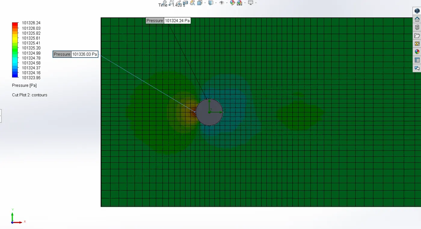
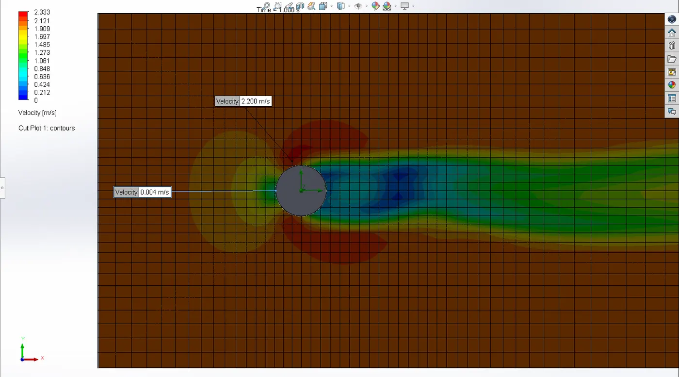
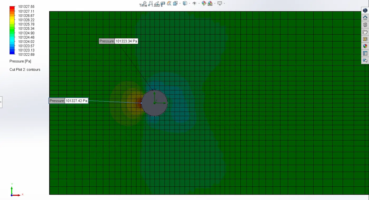
Observing the above Cut Plots and animations, we can see that at the first point of contact between fluid and cylinder i.e at 0° on the curved surface of cylinder, the fluids comes at rest , velocity is minimum or zero and pressure is maximum. This is the Stagnation point.
Then the velocity goes on increasing and pressure goes on decreasing in first half of cylinder. The point of maximum velocity at which boundary layer seperation starts is called Seperation point. In this case its seen around at 90° and 270° on curved surface of cylinder.
Further now the pressure agains starts increasing that is Adverse Pressure Gradient and as a result fluid starts flowing reverse or comes to rest. This gives rise to Wake region behind the cylinder which causes drag effect.
We can also see that as Seperation of boundery layer takes places due to unstable shear layer , vortices are seen formed and moving away from cylinder.Also it is evident that at the start vortices are formed alternately at top and bottom surfaces as change in velocities and pressures can be observed at that places in animations. This is what leads to Vortex Shedding.

Though this Observations are common in all the cases , yet as the Reynolds number increasing we can see that Seperation point shifts forward along the cylinder which leads to lesser wake region. Thus more turbulent flow is preferable to reduce drag effect.

Reference:

http://farside.ph.utexas.edu/teaching/336L/Fluidhtml/node116.html