Week 3 - Solving second order ODEs

AIM : To write a program to simulate simple pendulum motion.

OBJECTIVES :

• Writing a program to simulate simple pendulum motion with damping using

Length of the string : L = 1 metre,

Mass of the Pendulum : m = 1 kg,

Damping Coefficient : b = 0.05,

Gravity : g = 9.81 m/s square.

Motion between 0-20 sec, for angular displacement=0,angular velocity=3 rad/sec at time t=0

THEORY : A simple pendulum is one which can be considered to be a point mass suspended from a string or rod of negligible mass. It is a resonant system with a single resonant frequency.

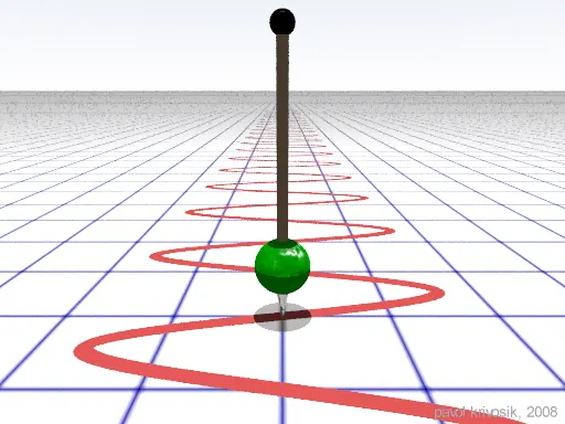
The position of the simple pendulum (Theta) with respect to time can be determined by using a 2nd order differential equation using Matlab/Octave.The Theta value can be solved breaking the 2nd order differential equation to the first order differential equation. Matlab/Octave follow Runge-Kutta fourth order method.

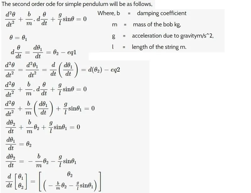
FUNCTION PROGRAM :

function [dtheta_dt]=ode_func(t,theta,b,g,l,m)
  
  theta1=theta(1)
  theta2=theta(2)
  dtheta1_dt = theta2;
  dtheta2_dt = -(b/m)*theta2 - (g/l)*sin(theta1);
  dtheta_dt = [dtheta1_dt; dtheta2_dt];
   
 end

PROGRAM :

clear all
close all
clc 

l=1                 %Length of string
m=1                 %Mass of Pendulum
b=0.05              %Damping Coeff
g=9.81              %Gravity

%Initial Condition
theta_0=[0;3];      %angular velocity 3rad/sec

%Time Points
t_span= linspace(0,20,200);   %0-20 Sec


%Solving ODE
[t,results]=ode45(@(t,theta) ode_func(t,theta,b,g,l,m),t_span,theta_0);
      
figure(1)
plot(t,results(:,1),'color','r');
hold on
plot(t,results(:,2),'color','b');
ylabel('Displacement & Angular Velocity')
legend('Displacement','Angular Velocity')
xlabel('time')
 
ct=2
 for i=1:length(results(:,1))
   x1=-1*sin(results(i,1));
   y1=-1*cos(results(i,1));
   
   figure(ct)
   plot([0,x1],[0,y1],'linewidth',1)    % Plotting a string with width line of 1
   hold on
   plot(x1,y1,'o','color','r');         % Plotting a bob
   hold off
   grid on;
   axis([-1.5 1.5 -1.5 1.5])            % Mentioning axis to show plot
   pause(0.006);
   file=sprintf('Pendulum%d.png',ct)    % Printing and naming the png file
   saveas(gca,file)                     % Calling png files to save
   ct=ct+1;
 end

RESULTS :

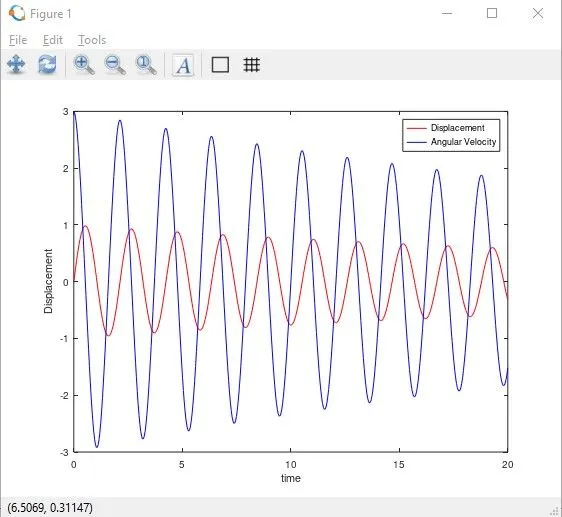
Plotting Displacement Vs Angular Velocity

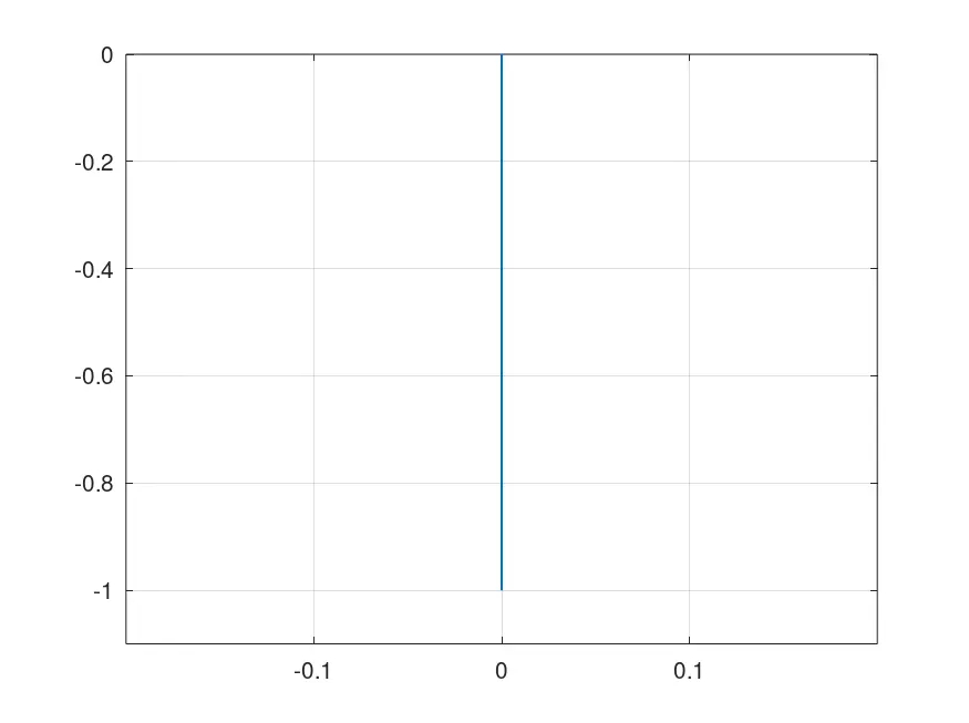
• Simple Pendulum Animation

CONCLUSION : By using ODE45 function we were able to find the theta for 2nd order differential equation for a simple pendulum and creating animation of the same. we can see that if we increase the damping value the displacement and angular velocity goes decreasing simultaneously as time increases.