Week 3 - Solving second order ODEs

AIM: To simulate the motion of a pendulum by solving a second-order differential equation in MATLAB

INPUTS PROVIDED:

• Length of pendulum:1m
• Mass = 1kg
• Damping Co-efficient: 0.05
• Acceleration due to gravity: 9.81 m/s^2
• At time =0; angular displacement=0 and angular velocity=3 rad/sec
• Total time of observation: 20 sec

CODE:

close all
clc

%Inputs provided
b=0.05; %Damping co-effecient
g=9.81; % Acceleration due to gravity (m/sec)
l=1; % lenght of pendulum in meter
m=1; % Pendulum mass in kg

%Defining initial Condition
%Angular Displacement=0
%Angluar Velovity=3 rad/s
theta_0=[0;3];

%Time points
time_span=linspace(0,20,500); % zero to 20 sec with 500 steps inbetween

%Solve ODE
[t,results]=ode45(@(time_span,theta) ode_func(time_span,theta,b,g,l,m),time_span,theta_0);

%Plotting the results linearly
figure(1)
plot(t,results(:,1))
hold on
plot(t,results(:,2))
ylabel('Plot')
xlabel('Time(s)')
legend('Displacement','Angular Velocity');
hold off

theta2=results(:,1);%Separating results for mapping
count=1; %counter for looping
% Defining the origin point for the pendulum 
x_init = 0;
y_init = 0;
for i=1:length(theta2)
    
    theta=theta2(i);
    
    %Finding co-ordinates from theta values  
    x=l*sin(theta);
    y=-l*cos(theta);
    
    figure(2);
    axis equal;
    cla;
    plot(0,0,'*','markers',10);
    hold on
    plot([x_init x],[y_init y],'color','b');
    hold on
    plot(x,y,'o','markers',15,'markerfacecolor','g');
    grid on;
    title('Pendulum');
    axis([-1.5 1.5 -1.5 0]);
    M(i)=getframe(gcf);
    count=count+1;
end
%Saving the video file
hold off;
movie(M)
videofile=VideoWriter('ode45_pendulum.avi','Uncompressed AVI');
open(videofile);
writeVideo(videofile,M);
close(videofile);

% Function for ODE45
function [dtheta_dt] = ode_func(~,theta,b,g,l,m)
    theta1=theta(1);
    theta2=theta(2);
    dtheta1_dt=theta2;
    dtheta2_dt=-(b/m)*theta2-(g/l)*sin(theta1);
    dtheta_dt=[dtheta1_dt; dtheta2_dt];
end

OUTPUTS:

Figure 1 shows the variation of angular velocity and displacement with respect to time. The effect of the damping coefficient can be clearly seen as the amplitude keeps on reducing. If the observation time were to be a little more, the reduction of the amplitude to zero can be seen. Figure 2 shows the movement of the pendulum for the values from figure 1.

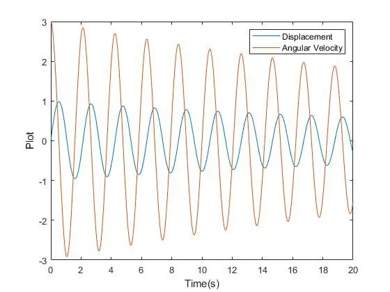
Figure 1: Plot showing the change in displacement and velocity as a function of time.

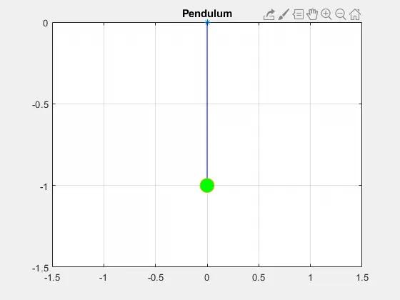
Figure 2: Pendulum animation

CONCLUSION: A successful implementation of the second-order differential equation was used to solve the motion of the pendulum. The displacement, as well as the acceleration, was plotted and the animation of the motion of the pendulum was shown. The same techniques can be applied to calculate the spring-mass damper systems and similar systems such as that.

ERRORS FACED:

Multiple errors were faced while writing the loop for the simulation for the motion of the pendulum. But it was trial and error to make the loop work. Unfortunately, I was not able to take any images of the errors. There were errors while saving the video file as well but I was able to get it working in the end.