Project 2 - Rankine cycle Simulator

AIM: To simulate a Rankine cycle in MATLAB

Code Explanation:

• The program takes in inputs from the user. Three major inputs are provided which is boiler pressure, condenser pressure and the turbine inlet temperature. It is to be noted that this program utilizes an external steam library called XSteam.
• The program outputs the state variables at all the main stages and state variables such as enthalpy, entropy, pressure, and temperature are also calculated. Along with this, the net-work and the back work ratio of the cycle are also calculated.
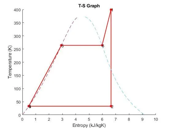
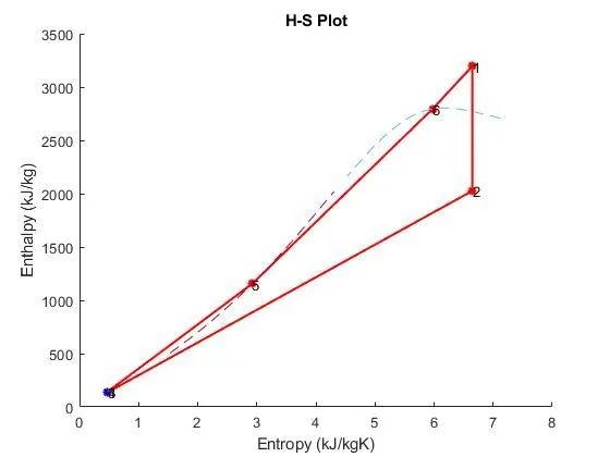
• All of the calculations are plotted in two graphs - Enthalpy vs. Entropy and Temperature vs. Entropy. The liquid and the vapour saturation lines are also plotted for better understanding.

Code:

clear
clc

%Inputs for the calculation
%Pressure at turbine entrance/boiler pressure
p_1 = str2double(input('Enter the boiler pressure in Bar(s) (number only): ','s'));

%Temperature at turbine entrance
t_1 = str2double(input('Enter the turbine entrance temperature in Degree celcius (number only): ','s'));

%Pressure at turbine exit/condenser pressure
p_2 = str2double(input('Enter the condenser pressure in bar(s) (number only): ','s'));

%Saturation temperature at boiler pressure
t_sat = XSteam('tSat_p',p_1);

%Step to determine the turbine has saturated or superheated steam

if(t_sat==t_1) %saturated
    h_1 = XSteam('hV_p',p_1);
else %super-heated
    h_1 = XSteam('h_pt',p_1,t_1);
end

%Entropy at turbine entrance
s_1 = XSteam('s_pt',p_1,t_1);

%As, expansion in a steam turbine is an isentropic process
s_2 = s_1; %Entropy at turbine exit

%Steam is supposed to be wet steam after turbine phase
sf_2 = XSteam('sL_p',p_2); %saturated liquid entropy at 0.05 bars

sg_2 = XSteam('sV_p',p_2); %saturated vapour entropy at 0.05 bars

x_2 = (s_2 - sf_2)/(sg_2-sf_2); %dryness fraction of the wet steam at turbine exit

h_g2 = XSteam('hV_p',p_2); %enthalpy of saturated steam at condenser pressure

h_f2 = XSteam('hL_p',p_2); %enthalpy of saturated liquid at condenser pressure

h_2 = h_f2 + x_2*(h_g2 - h_f2); %enthalpy of mixed steam at turbine exit

%mixed steam after passing through the condenser becomes saturated liquid
h_3 = XSteam('hL_p',p_2); %enthalpy of liquid at condenser exit

%Pump is an open system where the liquid pressure is increased and it
%becomes supercooled. Since the pump compartment volume remains constant, it is isochoric
vol_3 = XSteam('vL_p',p_2); %specific volume of saturated liquid at condenser pressure

%work done by pump 
work_pump = vol_3*(p_1-p_2)*10^2; %flow work done by pump as it is an open system

h_4 = h_3 + work_pump; %enthalpy of liquid at boiler entrance/pump exit

work_turbine = h_1-h_2; %work done by turbine

%Net Work
work_net = work_turbine - work_pump; %work done by turbine = work done by the system + work done by the pump

back_work_ratio = work_turbine/work_pump; %back work ratio = work produced by turbine/work consumed by pump

%STATE 1 VARIABLES

fprintf('The state variables of State 1 are:\n')
fprintf('Enthalpy (kJ/kg) = %f\n',h_1)
fprintf('Entropy (kJ/kgK)= %f\n',s_1)
fprintf('Temperature (deg.C) = %f\n',t_1)
fprintf('Pressure (bars) = %f\n',p_1)

%STATE 2 VARIABLES

t_2 = XSteam('t_ph',p_2,h_2);
fprintf('The state variables of State 2 are:\n')
fprintf('Enthalpy (kJ/kg) = %f\n',h_2)
fprintf('Entropy (kJ/kgK) = %f\n',s_2)
fprintf('Temperature (K) = %f\n',t_2)
fprintf('Pressure (bars) = %f\n',p_2)

%STATE 3 VARIABLES
%h_3
s_3 = XSteam('sL_p',p_2);
%p_2
t_3 = XSteam('t_ph',p_2,h_3);%ideally t_3 = t_2
fprintf('\n The state variables of State 3 are:')
fprintf('\n Enthalpy (kJ/kg) = %f',h_3)
fprintf('\n Entropy (kJ/kgK) = %f',s_3)
fprintf('\n Temperature (K) = %f',t_3)
fprintf('\n Pressure (bars)= %f',p_2)

%STATE 4 VARIABLES
%h_4
s_4 = XSteam('s_ph',p_1,h_4);%ideally pump process is isentropic
%p_1
t_4 = XSteam('t_ph',p_1,h_4);
fprintf('The state variables of State 4 are:')
fprintf('\n Enthalpy (kJ/kg) = %f',h_4)
fprintf('\n Entropy (kJ/kgK) = %f',s_4)
fprintf('\n Temperature (K)= %f',t_4)
fprintf('\n Pressure (bars) = %f',p_1)

fprintf('\n Net work done by the cycle is: %f',work_net)
fprintf('\n Back work ratio of the cycle is: %f \n',back_work_ratio)

%Intermediate stages in boiler
%economiser stage
h_5 = XSteam('hL_p',p_1);
s_5 = XSteam('sL_p',p_1);
t_5 = XSteam('t_ph',p_1,h_5);

%superheat stage
h_6 = XSteam('hV_p',p_1);
s_6 = XSteam('sV_p',p_1);
t_6 = XSteam('t_ph',p_1,h_6);

%Plotting the saturation dome for T-S plot
T = (0:2:374);
svap = arrayfun(@(t) XSteam('sV_t',t),T);
sliq = arrayfun(@(t) XSteam('sL_t',t),T);

%Plotting the saturation curve for H-S plot
P = (0:2:300);
sliq1 = arrayfun(@(p) XSteam('sL_p',p),P);
hliq = arrayfun(@(p,s) XSteam('h_ps',p,s),P,sliq1);
svap1 = arrayfun(@(p) XSteam('sV_p',p),P);
hvap = arrayfun(@(p,s) XSteam('h_ps',p,s),P,svap1);

%T-S Plot
figure(1)
hold on
plot([s_1 s_2],[t_1 t_2],s_2,t_2,'*','linewidth',1.5,'color','r')
plot([s_2 s_3],[t_2 t_3],s_3,t_3,'*','linewidth',1.5,'color','r')
plot([s_3 s_4],[t_3 t_4],s_4,t_4,'*','linewidth',1.5,'color','r')
plot([s_4 s_5],[t_4 t_5],s_5,t_5,'*','linewidth',1.5,'color','r')
plot([s_5 s_6],[t_5 t_6],s_6,t_6,'*','linewidth',1.5,'color','r')
plot([s_6 s_1],[t_6 t_1],s_1,t_1,'*','linewidth',1.5,'color','r')
plot(svap,T,'--')
plot(sliq,T,'--')
text(s_1,t_1,'1')
text(s_2,t_2,'2')
text(s_3,t_3,'3')
text(s_4,t_4,'4')
text(s_5,t_5,'5')
text(s_6,t_6,'6')
xlabel('Entropy (kJ/kgK)')
ylabel('Temperature (K)')
title('T-S Graph')

%H-S Plot
figure(2)
hold on
plot([s_1 s_2],[h_1 h_2],s_2,h_2,'*','linewidth',1.5,'color','r')
plot([s_2 s_3],[h_2 h_3],s_3,h_3,'*','linewidth',1.5,'color','r')
plot([s_3 s_4],[h_3 h_4],s_4,h_4,'*','linewidth',1.5,'color','b')
plot([s_4 s_5],[h_4 h_5],s_5,h_5,'*','linewidth',1.5,'color','r')
plot([s_5 s_6],[h_5 h_6],s_6,h_6,'*','linewidth',1.5,'color','r')
plot([s_6 s_1],[h_6 h_1],s_1,h_1,'*','linewidth',1.5,'color','r')
text(s_1,h_1,'1')
text(s_2,h_2,'2')
text(s_3,h_3,'3')
text(s_4,h_4,'4')
text(s_5,h_5,'5')
text(s_6,h_6,'6')
plot(svap1,hvap,'--')
plot(sliq1,hliq,'--')
xlabel('Entropy (kJ/kgK)')
ylabel('Enthalpy (kJ/kg)')
title('H-S Plot')

%Plotting the saturation dome for T-S plot
T = (0:2:374);
svap = arrayfun(@(t) XSteam('sV_t',t),T);
sliq = arrayfun(@(t) XSteam('sL_t',t),T);

%Plotting the saturation curve for H-S plot
P = (0:2:300);
sliq1 = arrayfun(@(p) XSteam('sL_p',p),P);
hliq = arrayfun(@(p,s) XSteam('h_ps',p,s),P,sliq1);
svap1 = arrayfun(@(p) XSteam('sV_p',p),P);
hvap = arrayfun(@(p,s) XSteam('h_ps',p,s),P,svap1);

Outputs: