Week - 2 - Explicit and Implicit Analysis
Explicit Analysis:
Explicit analysis is used to non-linear type of analysis and can be calculated with relative ease. Since small time steps are necessary for such an analysis which results in good accuracy it is mostly used for dynamic analysis.
Equation: F(u) = u^3+9u^2+4x
Solution:
K(u) = dF/du = 3u^2+18u+4
WKT, ∆F = k∆u
- U1 = 0.0 -> k(u0) = 1, ∆F = 1
K(u0) = 0+0+4 = 4
∆u1 = ∆F/k(u0) = ¼ = 0.25
U1 = u0 + ∆u1 = 0 + 0.25 = 0.25
- U1 = 0.25
K(u1) = 3*(0.25)^2 + 18(0.25) + 4 = 8.6875
∆F = 1
∆u2 = ∆F/k(u1) = 1/8.6875 = 0.1151
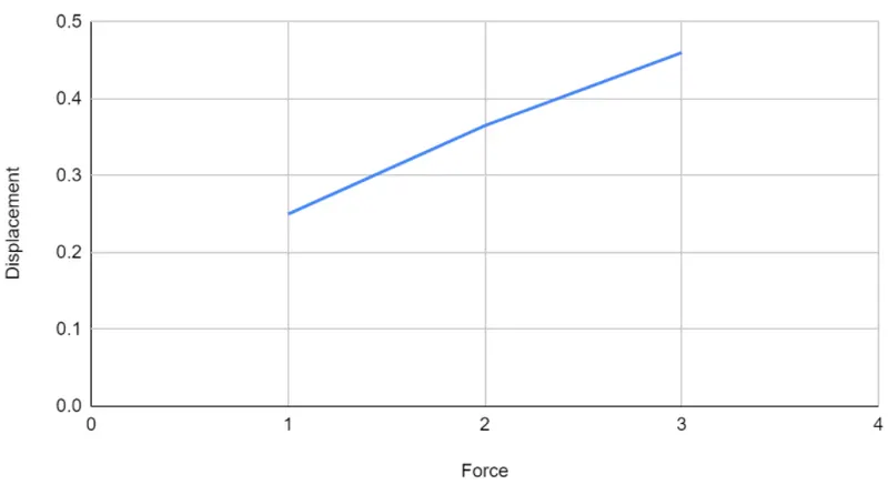
U2 = u1 + ∆u2 = 0.3651
- U2 = 0.3651
K(u2) = 3*(0.3651)^2 + 18(0.3651) + 4 = 10.9716
∆F = 1
∆u3 = ∆F/k(u2) = 1/10.9761 = 0.09114
U3 = u2 + ∆u3 = 0.45625
F_ext = ∆F + ∆F + ∆F = 3.0
F_int = (0.45624)^2 + 9*(0.4562)^2 + 4*(0.4562) = 3.79
Therefore, F_ext ≠ F_int
|
Step i |
∆Fi |
∆ui |
Ui |
F_exti |
F_inti |
R = F_inti-F_exti |
|
1 |
1 |
0.25 |
0.25 |
1 |
1.528 |
0.578 |
|
2 |
1 |
0.1131 |
0.3651 |
2 |
2.708 |
0.708 |
|
3 |
1 |
0.09114 |
0.45624 |
3 |
3.891 |
0.841 |
Force vs. Displacement:
Implicit Analysis:
The implicit analysis uses the Newton_rhapson method in order to perform iterations to reach the tolerance limit and hit equilibrium. This process on a computer utilizes matrix inversion and hence is computationally expensive when compared to explicit type analysis. They also do not have a time-step size and hence can be several times larger than what is used for explicit analysis.
Equation: F9u) = u^3 + 9u^2+4u ---(1)
Stiffness: K(u) = dF/du = 3u^2 + 18u+4 ----(2)
Tolerance: 10^-2
Step 1:
U0 = 0, eqn. 2 becomes: k(u0) = 3(0)^2 + 18(0) +4 = 4
∆u1 = ∆F/k(u0) = ¼ = 0.25
U1 = u0=∆u1 = 0+0.25 = 0.5
Check residual, F_ext = ∆F = 1; f_int = (0.25)^3+9(0.25)^2+4(0.25) = 1.578
R(0) = f_int – F_ext = 1.578 -1 = 0.578 > 10^-2
Tolerance requirements not met.
Newton-Rhapson iteration necessary.
Calculating correction to u1 = u1(0):
∂u(1) = -[ku1(0)]^-1 * R_0 = [3(0.25)^3+18(0.25)^2+4]^-1*0.578 = -0.0665
Updated value u1(1) = u1^(0) + ∂u^(1) = 0.25 – 0.665 = 0.1835
Check residual again,
F_ext= 1; f_int = (0.1835)^3+9(0.1835)^2+4(0.1835) = 1.0438
R(1) = f_int – F_ext = 1.0432 – 1 = 0.0432 >10^-2
Another iteration needed.
Calculating correct to u1 = u1(1)
∂u(2) = ∂u(1) – [ku1(1)]^-1 * R1 = [-0.0665 – 8.6875]^-1 * 0.0432 = -0.0714
U1(2) = u1(1) + ∂u(2) = 0.25 – 0.0714 = 0.1786
Check residual – R2:
F_est = 1, f_int = (0.1786)^3 + 9(0.1786)^2 + 4(0.1786) = 1.0071
R2 = 1.0071 -1 = 0.0071 <10^-2
Therefore, u1 = 0.1786
Similarly,
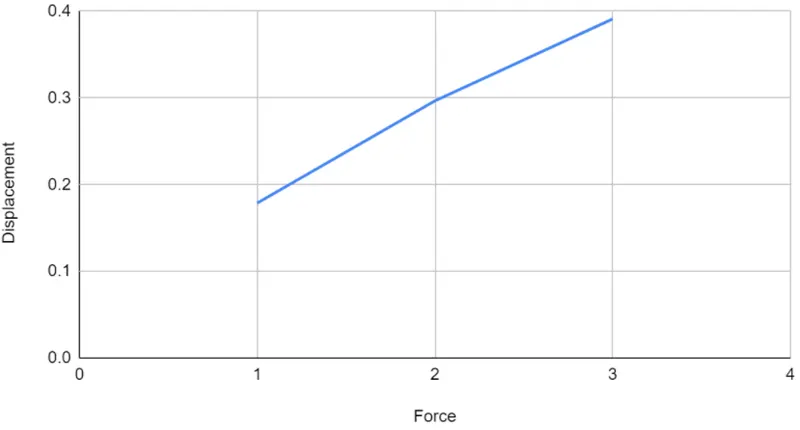
U2 = 0.2966
U3 = 0.3911
|
Step i |
∆Fi |
∆ui |
Ui |
F_exti |
F_inti |
R = F_inti-F_exti |
|
1 |
1 |
0.25 |
0.1786 |
1 |
1.0071 |
0.0071 |
|
2 |
1 |
0.1374 |
0.2966 |
2 |
2.0042 |
0.0042 |
|
3 |
1 |
0.1041 |
0.3911 |
3 |
3.0008 |
0.0008 |
Force vs. Displacement: