Week 3 -Simulation and Animation of a Simple Pendulum motion using Matlab.

AIM:

g = gravity in m/s2, L = length of the pendulum in m, m = mass of the ball in kg, b=damping coefficient.

Write a program in Matlab that will simulate the pendulum motion.

use,

L=1 metre,

m=1 kg,

b=0.05.

g=9.81 m/s2.

Simulate the motion between 0-20 sec, for angular displacement=0,angular velocity=3 rad/sec at time t=0.

When you do this you will get the position of the pendulum as a function of time. Use this information to animate the motion of the pendulum, as shown in the below figure.

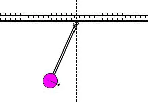
Your animation does not have to look exactly like this and here is the logic.

• For each value in time
• Create an image that represents the position of the pendulum
• You can assume the length of the string and the size of the ball
• Use the marker command to create a sphere
• One end of the pendulum is fixed
• The other end moves according to the solution of the ODE you had solved.
• If you are using Matlab, use the movie command to create an animation

________________________________________________________________________________________________________________________________________________________________________________________________

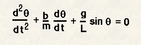
ODE Equation:

________________________________________________________________________________________________________________________________________________________________________________________________

code for ode_function:

function [dtheta_dt]=ode_f(t,theta,b,g,l,m)
theta1=theta(1)
theta2=theta(2)
dtheta1_dt=theta2;
dtheta2_dt=-(b/m)*theta2-(g/l)*sin(theta1);
dtheta_dt=[dtheta1_dt;dtheta2_dt]
end

________________________________________________________________________________________________________________________________________________________________________________________________

Main Code:

%inputs
b=0.05;
g=9.81;
l=1;
m=1;
%intial conditions [ displacement, velocity]
theta_DV=[0;3];
t_span=linspace(0,20,500);
%calling function
[t,results]=ode45(@(t,theta)ode_f(t,theta,b,g,l,m),t_span,theta_DV);
figure(1)
plot(t,results(:,1),'linewidth',0.8,'color','b')
hold on;
plot(t,results(:,2),'linewidth',0.8,'color','r')
xlabel('time-sec')
ylabel('displacement and angular velocity')
legend('change in displacement','change in angular velocity')
hold off

figure(2)
plot(results(:,1),results(:,2))
xlabel('position-radians')
ylabel('Angular velcoity')

figure(3)
ct=1;
for i=1:length(t)
theta1=results(:,1);
THETA1=theta1(i);
%coordinates
x0=0;
y0=0;
x1=l*sin(THETA1);
y1=-l*cos(THETA1);
%ploting
plot([x0 x1],[y0 y1],'color','b','linewidth',2)
hold on
plot([-1.1 1.1],[0 0],'linewidth',2)
plot(x1,y1,'o','markersize',20,'markerfacecolor','r')
hold off
grid on
axis([-1.5 1.5 -1.5 0.5])
M(ct)=getframe(gcf);
pause(0.003)
ct=ct+1;
end
movie(M)
videofile=VideoWriter('simple_pendulum.avi','uncompressed AVI');
open(videofile)
writeVideo(videofile,M)
close(videofile)

________________________________________________________________________________________________________________________________________________________________________________________________

Explanation:

*Defining the inputs for damping, gravity, length, and mass (b, g, l, and m).

*Defining initial conditions, Since there are two first-order ode systems, one for displacement and another for velocity.

theta_DV=[0;3];

*Next I am integrating the ode system to obtain a solution. Hence we define the values for time(seconds).

t_span=linspace(0,20,500);

*Then we call our ode function, where ode 45 is an inbuilt function with [t, theta] as the dependent and independent variables, then we define our function: ode_f(b, g, l, m); then we provide the initial conditions, integration and the time array which say how far the integration needs to be done and then the initial conditions corresponding to the starting of the time which is theta_DV.

code for ode_f:

function [dtheta_dt]=ode_f(t,theta,b,g,l,m)
theta1=theta(1)
theta2=theta(2)
dtheta1_dt=theta2;
dtheta2_dt=-(b/m)*theta2-(g/l)*sin(theta1);
dtheta_dt=[dtheta1_dt;dtheta2_dt]
end

*This function in turn gives us the time and results [t, results]. then we plot a graph that shows the change in displacement and angular velocity with respect to time. then we plot another graph that shows the position and angular velocity using the results.

*Finally we create an animation for the simple pendulum and save the file and then we run and close the file.

________________________________________________________________________________________________________________________________________________________________________________________________