Project 2 - Rankine cycle Simulator
AIM:
- Create a Rankine Cycle Simulator using MATLAB.
- Your code should calculate the state points of the Rankine Cycle (any type of your choice) based on user inputs.
- Then, plot the corresponding T-s and h-s plots for the given set of inputs. Title and axes labels are a must, while legends could be used if necessary.
- Attach a report explaining the working of a Rankine cycle simulator and also the research done by you.
Theory:
- High Energy steam is developed in a boiler
- It is passed through a turbine to develop power
- The Exit steam from the turbine is passed to a condenser to convert it into liquid water.
- This liquid water is sent back to the Boiler with the help of a Pump. this liquid is passed to the Boiler for the generation of steam.
Process 1-2: Turbine
work is generated through the expansion of Vapour(isentropic Expansion).
Process 2-3: Condenser
Heat rejection occurs at constant pressure(Isobaric process).
Process3-4: Pump
constant Entropy process (isentropic Compression).
process 4-1: Boiler
Heat addition occurs at constant pressure(Isobaric process).
________________________________________________________________________________________________________________________________________________________________________________________________
Main Code:
T1=input('Enter the turbine inlet Temperature(celcius)\n');
p1=input('Enter the turbine inlet pressure(bars)\n');
p2=input('Enter the turbine outlet pressure(bars)\n');

%process 1-2 is isentropic expansion
%process 2-3 is constant pressure heat rejection
%process 3-4 is isentropic compression
%process 4-1 is constant pressure heat addition

%s=specific Entropy(s1,s2,s3,s4)
%Sl=saturated liquid entropy
%sg=saturated gas/vapour entropy
%h=specific Enthalpy(h1,h2,h3,h4)
%hl=saturated liquid enthalpy
%hg=saturated gas/vapour enthalpy

%variables at state point 1 (turbine)
h1=XSteam('h_pT',p1,T1);
s1=XSteam('s_pT',p1,T1);
sl1=XSteam('sL_p',p1);
sg1=XSteam('sV_p',p1);
hl1=XSteam('hL_p',p1);
hg1=XSteam('hV_p',p1);

%variables at state point 2 (condensor)
s2=s1;
sl2=XSteam('sL_p',p2);
sg2=XSteam('sV_p',p2);
hl2=XSteam('hL_p',p2);
hg2=XSteam('hV_p',p2);
X2=((s2-sl2)/(sg2-sl2)); %X is the dryness fraction
h2=(hl2+(X2*(hg2-hl2)));
T2=XSteam('T_ph',p2,h2);

%work done by turbine
%apply first law q=0, W=+ve
%h+q=h+W || h1-h2=Wt
W_turbine=h1-h2;

%variables at state point 3 (pump)
T3=T2;
p3=p2;
h3=hl2;
s3=sl2;

%variables at state point 4 (boiler)
s4=s3;
p4=p1;
h4=XSteam('h_ps',p4,s4);
T4=XSteam('T_ps',p4,s4);
%properties of intermediate points b/w pts 4-1
T5=XSteam('Tsat_p',p1);
p5=p1;
h5=XSteam('hL_P',p1);
s5=XSteam('sL_p',p1);

T6=XSteam('Tsat_p',p1);
p6=p1;
h6=XSteam('hV_P',p1);
s6=XSteam('sV_p',p1);

%heat Flow rate to or from the system(Qin/Qout)
Qin=h1-h4;
Qout=h2-h3;
%work done by pump
W_pump=h4-h3;

%net work done
Wnet= W_turbine-W_pump;
%back work ratio
back_wr=W_pump/W_turbine;
%efficiency(eff)
eff=Wnet/Qin;
%Specific Steam Consumption(SSC)
ssc=3600/Wnet;
%Outputs
%properties at point 1
fprintf('T1=%f celcius\n',T1);
fprintf('p1=%f bars\n',p1);
fprintf('h1=%f KJ/Kg\n',h1);
fprintf('s1=%f KJ/kgC\n',s1);
%properties at point 2
fprintf('T2=%f celcius\n',T2);
fprintf('p2=%f bars\n',p2);
fprintf('h2=%f KJ/Kg\n',h2);
fprintf('s2=%f KJ/kgC\n',s2);
%properties at point 3
fprintf('T3=%f celcius\n',T3);
fprintf('p3=%f bars\n',p3);
fprintf('h3=%f KJ/Kg\n',h3);
fprintf('s3=%f KJ/kgC\n',s3);
%properties at point 4
fprintf('T4=%f celcius\n',T4);
fprintf('p4=%f bars\n',p4);
fprintf('h4=%f KJ/Kg\n',h4);
fprintf('s4=%f KJ/kgC\n',s4);
fprintf('______________results_______________\n');
fprintf('net work done by the system = %f (KJ/KG)\n',Wnet);
fprintf('back word ratio = %f\n',back_wr);
fprintf('efficiency of the cycle = %f %\n',eff);
fprintf('specific steam consumption = %f (kG/K.W.hr)\n',ssc);
%ploting saturation lines
T=(1:2000);
for i=1:1:2000
    sL(1,i)=XSteam('sL_T',i);
    sV(1,i)=XSteam('sV_T',i);
    hL(1,i)=XSteam('hL_T',i);
    hV(1,i)=XSteam('hV_T',i);
end
figure(1)
plot(sL,T,'b','linewidth',1);
hold on
plot(sV,T,'b','linewidth',1);
xlabel('Entropy (KJ/kG.c)');
ylabel('Temperature.^(C)');
title('temperature vs entropy')
figure(2)
plot(sL,hL,'b','linewidth',1);
hold on
plot(sV,hV,'b','linewidth',1);
xlabel('Entropy (KJ/kG.C)');
ylabel('Enthalpy (KJ/KG)');
title('Entropy vs Enthalpy');
%plotting Rankine cycle
figure(1)
plot([s1,s2,s3,s4,s5,s6,s1],[T1,T2,T3,T4,T5,T6,T1],'k','linewidth',1)
figure(2)
plot([s1,s2,s3,s4,s5,s6,s1],[h1,h2,h3,h4,h5,h6,h1],'k','linewidth',1)
________________________________________________________________________________________________________________________________________________________________________________________________
Explanation:
The user inputs are coded= enter the values of temperature, the pressure at inlet, and exit of the turbine as given in the question.

T1=input('Enter the turbine inlet Temperature(celcius)\n');
p1=input('Enter the turbine inlet pressure(bars)\n');
p2=input('Enter the turbine outlet pressure(bars)\n');
next using the XSteam table find
1 the specific enthalpy(h1) with respect to pressure(p1) and temperature(T1)
2 the specific entropy(s1) with respect to pressure(p1) and temperature(T1)
3 the saturated liquid entropy(sl1) with respect to pressure(p1)
4 the saturated Vapour entropy(sg1) with respect to pressure(p1)
5 the saturated liquid enthalpy(hl1) with respect to pressure(p1)
6 the saturated Vapour enthalpy(hg1) with respect to pressure(p1)


%variables at state point 1 (turbine)
h1=XSteam('h_pT',p1,T1);
s1=XSteam('s_pT',p1,T1);
sl1=XSteam('sL_p',p1);
sg1=XSteam('sV_p',p1);
hl1=XSteam('hL_p',p1);
hg1=XSteam('hV_p',p1);
using XSteam derive the equations for state variables 2 just like state variables 1
1 since its isentropic process s2=s1.
2 calculate the saturated liquid entropy(sl2)
3 calculate the saturated Vapour entropy(sg2)
4 calculate the saturated liquid enthalpy(hl2)
5 calculate the saturated Vapour enthalpy(hg2)
6 calculate the dryness fraction(X)
7 finally we can find the specific enthalpy and temperature at state point 2
8 then calculate the work done by the turbine by calculating the difference in enthalpy.

%variables at state point 2 (condensor)
s2=s1;
sl2=XSteam('sL_p',p2);
sg2=XSteam('sV_p',p2);
hl2=XSteam('hL_p',p2);
hg2=XSteam('hV_p',p2);
X2=((s2-sl2)/(sg2-sl2)); %X is the dryness fraction
h2=(hl2+(X2*(hg2-hl2)));
T2=XSteam('T_ph',p2,h2);

%work done by turbine
%apply first law q=0, W=+ve
%h+q=h+W || h1-h2=Wt
W_turbine=h1-h2;
similarly derive and calculate the equations and find the variables for all state and intermediate points in the cycle

%variables at state point 3 (pump)
T3=T2;
p3=p2;
h3=hl2;
s3=sl2;

%variables at state point 4 (boiler)
s4=s3;
p4=p1;
h4=XSteam('h_ps',p4,s4);
T4=XSteam('T_ps',p4,s4);

%properties of intermediate points b/w pts 4-1
T5=XSteam('Tsat_p',p1);
p5=p1;
h5=XSteam('hL_P',p1);
s5=XSteam('sL_p',p1);

T6=XSteam('Tsat_p',p1);
p6=p1;
h6=XSteam('hV_P',p1);
s6=XSteam('sV_p',p1);
Then after finding all the state point variables we can calculate
1 The heat flow rate
2 The net-work done
3 The back work ratio
4 The efficiency of the cycle
5 Specific steam consumption
%heat Flow rate to or from the system(Qin/Qout)
Qin=h1-h4;
Qout=h2-h3;
%work done by the pump
W_pump=h4-h3;
%net work done
Wnet= W_turbine-W_pump;
%back work ratio
back_wr=W_pump/W_turbine;
%efficiency(eff)
eff=Wnet/Qin;
%Specific Steam Consumption(SSC)
ssc=3600/Wnet;Then finally we can print the outputs using fprintf command and print the values in the command window to get a clear output.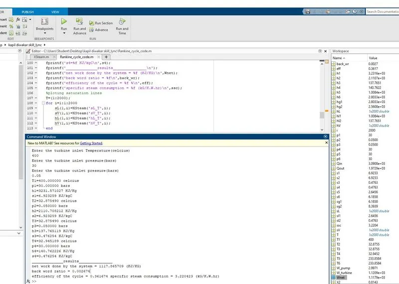
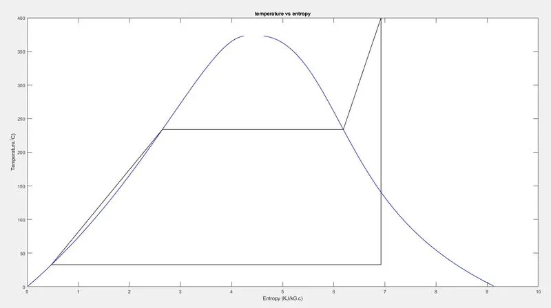
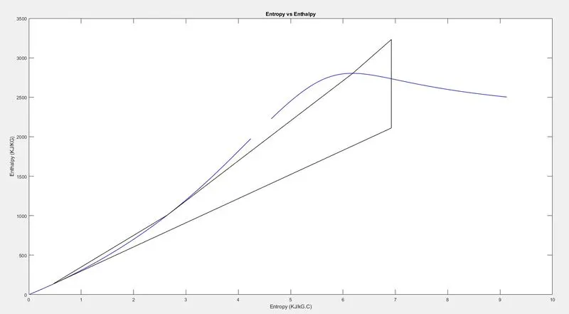
then plot the graphs for T-s and h-s
create an array
create a for loop for the saturation of liquid and gas lines between a range mentioned
plot the saturation lines for liquid and Vapour with respect to Temperature and Entropy and Entropy and Enthalpy of liquid/vapour.

Finally, create the Rankine cycle graph
plot the temperature vs Entropy points in figure(1)
plot the entropy vs enthalpy points in figure (2)

%ploting saturation lines
T=(1:2000);
for i=1:1:2000
    sL(1,i)=XSteam('sL_T',i);
    sV(1,i)=XSteam('sV_T',i);
    hL(1,i)=XSteam('hL_T',i);
    hV(1,i)=XSteam('hV_T',i);
end
figure(1)
plot(sL,T,'b','linewidth',1);
hold on
plot(sV,T,'b','linewidth',1);
xlabel('Entropy (KJ/kG.c)');
ylabel('Temperature.^(C)');
title('temperature vs entropy')
figure(2)
plot(sL,hL,'b','linewidth',1);
hold on
plot(sV,hV,'b','linewidth',1);
xlabel('Entropy (KJ/kG.C)');
ylabel('Enthalpy (KJ/KG)');
title('Entropy vs Enthalpy');
%plotting Rankine cycle
figure(1)
plot([s1,s2,s3,s4,s5,s6,s1],[T1,T2,T3,T4,T5,T6,T1],'k','linewidth',1)
figure(2)
plot([s1,s2,s3,s4,s5,s6,s1],[h1,h2,h3,h4,h5,h6,h1],'k','linewidth',1)
Reference video.https://www.youtube.com/watch?v=0udTK6hc6pQ
Reference Article:https://en.wikipedia.org/wiki/Rankine_cycle