Week 3 - Solving second order ODEs

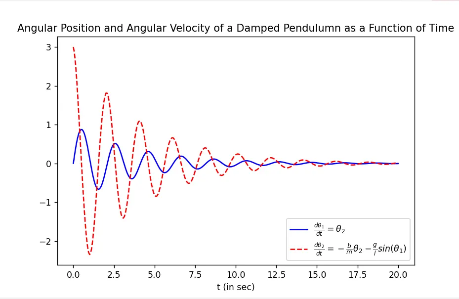
Objective: To plot the angular velocity and the angular displacement of a damped pendulum with respect to time using a code written in Python.

Explanation and Procedure:

ODEs are omnipresent in engineering problems as they play the major part in describing transient phenomena.

The equation of motion derived from Newton’s second law for a damped pendulum:

`d^2(theta)/(dt^2)+b/m*(d(theta)/dt)+g/l*sin(theta)=0`

Where,

“`theta`” describes the angular position, “b” is the damping constant, “m” is the mass of the bob, “l” is the length of the pendulum and “g” is the acceleration due to gravity.

For solving higher order ODEs using “odeint”, we need to break them into first order ODEs.

The equation of motion of the pendulum can be written in the form of two first order ODEs:

Let, `theta_1=theta`

`(d(theta_1))/dt=theta_2 `

`(d(theta_2))/dt=-b/m*((d(theta))/dt)-g/l*sin(theta)`

The ODE that will be solved by the code in matrix form;

`d/dt [(theta_1),(theta_2)]= [(theta_2),(-b/m(d(theta1))/dt-g/lsin(theta1))]`.

Firstly, a function has to be created that would take all the parameters regarding the oscillating system and return : `theta=[theta_1,theta_2].

In the code, this function is defined under the name “odefun”

The code: (with comments explaining each step)

import numpy as np

from scipy.integrate import odeint

import matplotlib.pyplot as plt

import math

#funcyion that return d(theta)/dt:

def odefun(theta,t,b,g,l,m):

theta1=theta[0]

theta2=theta[1]

dtheta1_dt=theta2

dtheta2_dt=-(b/m)*theta2-(g/l)*math.sin(theta1)

dtheta_dt=[dtheta1_dt,dtheta2_dt]

return dtheta_dt

#Inputs:

b=0.05 #(damping constant)

g=9.81 #(acceleration due to gravity)

l=1 #length of pendulumn

m=0.1 #mass of pendulumn

#Initial Conditions:

theta_i=[0,3]

#time

t_ndarray=np.linspace(0,20,300) #To simulate till 30 seconds with 300 time-steps

t=t_ndarray.tolist() #Type setting to a list.

#Solving the ODE:

theta=odeint(odefun,theta_i,t,args=(b,g,l,m))

#Plotting;

plt.plot(t,theta[:,0],'b-',label=r'$\frac{d\theta_1}{dt}=\theta_2$')

plt.plot(t,theta[:,1],'r--',label=r'$\frac{d\theta_2}{dt}=-\frac{b}{m}\theta_2-\frac{g}{l}sin(\theta_1)$')

plt.legend(loc='lower right')

plt.title("Angular Position and Angular Velocity of a Damped Pendulumn as a Function of Time")

plt.xlabel("t (in sec)")

plt.show()

The resulting plot: