Solving second order ODEs

Aim - Objective is to write a program that solves the following ODE

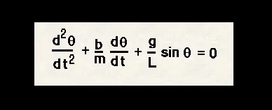
Theory -

We can solve a second order differential equation of the type , d²ydx² + P(x)dydx + Q(x)y = f(x) , where P(x), Q(x) and f(x) are functions of x, by using variation of parameters which only works when f(x) is a polynomial, exponential, sine, cosine or a linear combination of those.,undetermined coefficients which is a little messier but works on a wider range of function .

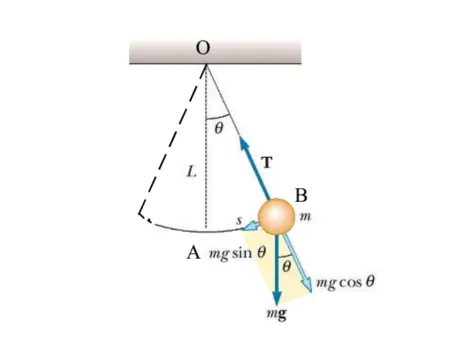
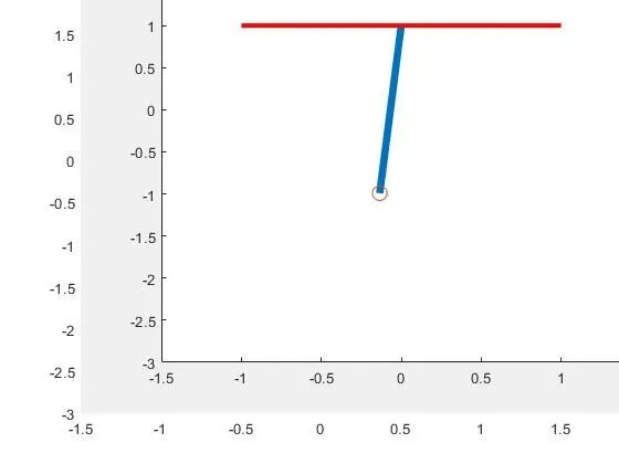
Simple pendulum diagram -

Procedure -

• We have to declare the basic inputs like damping (b),mass(m) , length (l)and gravity(g) they are as follows
  b=0.05;
  g=9.81;
  l=1;
  m=0.1;
• The % is used to show the comments , % initial conditions that is theta_0=[0;5] .
• Time points are given as shown %time points
  t_span = linspace(0,10,100) , in this the command linspace is used to display numbers between given outputs .
• to solve ode this code is required

  [t,results] = ode45(@(t,theta ) ode_function(t,theta,b,g,l,m),t_span,theta_0) . in which ode45 is a

  Ode45 is a function in matlab that solves ordinary or partial differential equations using a numerical method. The numerical method in question here is the 4th order Runge Kutta method.

• ode_function is a sub function which is defined by us in order to solve the sum it is not a pre defined program in matlab.

• The plots are given with the help of plot command .
• lable command is used to display comments on the graph .
• Grid on command is used to show the grid lines on the plot .
• The command legender is used to show angular displacement and angular velocity on the plot.

Code -

clear all 
close all
clc

b=0.05;
g=9.81;
l=1;
m=0.1;

%initial comditions
theta_0=[0;5];
%time points 
t_span = linspace(0,10,100);
%solve ode
[t,results] = ode45(@(t,theta ) ode_function(t,theta,b,g,l,m),t_span,theta_0);

plot(t,results(:,1))
hold on 
plot(t,results(:,2))
ylabel('plot')
xlabel('time')
grid on 
legend('angular displacement','angular velocity')
ct=1
for i=1:length(t)
    angle= results(:,1)
%     Angle = angle(1)
    x0 =0 ;
    y0 =1;
    x1 = 1*sin(angle(i));
    y1 = -1*cos(angle(i));
    figure(2)
   % hold on 
    plot([x0 x1 ],[y0 y1 ],'linewidth',5)
    line([-1,1],[1,1],'color','r','linewidth',3)
   %plot(x1,y1,'o','markersize',10)
    axis([-3 3 -3 3])
    M(ct)=getframe(gcf)
    hold off
    ct=ct+1;
end
Movie(M)
videofile = VideoWriter('ode_pendulum.avi','uncompressed AVI');
open(videofile)
writeVideo(videofile.M)
close(videofile)

Calling function code -

function [dtheta_dt] = ode_function(t,theta,b,g,l,m)

theta1=theta(1)
theta2=theta(2)
dtheta1_dt = theta2;
dtheta2_dt = -(b/m)*theta2-(g/l)*sin(theta1);
dtheta_dt =[dtheta1_dt ; dtheta2_dt]
end

Plots -

Figure 1 plot

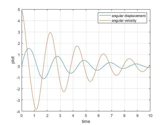
From this plot ve observe that angula velocity is starting from 5 and angular displacement is starting from 0 if it continiue further these two will merge at a certain point .

figure 2 plot

you tube link -

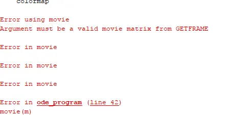
Errors in the code -