Week 3 - Solving second order ODEs

solving 2nd order differential quation.

Simple Pendulum

if we solve this equation we will be solving for this particular t which theta. so the rate at which the theta value is changing with respect to time (velocity).

In addition to this the pendulum also describe motion of a spring mass & damper system.

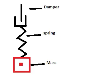
when we have higher order ODE we need to break it down into set of 1st order ODE.

d^2theta/dt+b/m dtheta/dt+g/l sintheta =0

b = damping

m = mass

g = gravity

l = length

theta = theta1

dtheta/dt = dtheta =theta2

d^2theta/dt^2 = d^theta/dt^2 = d/dt(dtheta/dt) = d/dt(theta)

d^2theta/dt^2+b/m dtheta/dt +g/l sintheta1

dtheta2/dt^+b/m dtheta2 +g/l sintheta1 = 0

dtheta1/dt = theta2 dtheta2/dt=b/m theta2-g/lsintheta1

d/dt[theta1/theta2] = [theta -b/mtheta2 -g/lsintheta]

Initial condition

theta = [0;5]

initial displacement is 0

initial velocity is 3m/s

we are going to integrating the ODE system to obtain a solution for which we need to define time.

time points

t_span = linespace(0,10,500)

we have to call the function

solve ODE

[t, results] = ode45(theta(t,theta)ode_function(t,theta,bglm)t_span,theta_0

plot(t,results(:,1))
hold on
plot(t,results(:,2))
xlabel('Plot')
ylabel('time')

ODE function is a seperate function that has been define to call it in programming and its input argument are deriving

theta1

theta2 

and then we are defining first order ODE

[dtheta_dt] = ode_func(t,theta,b,g,l,m)

theta1 = theta(1)
theta2 = theta(2)
dtheta1_dt = theta2;
dtheta2_dt = -(b/m)*theta2 -(g/l)*sin(theta1);
dtheta_dt = [ dtheta1_dt; dtheta2_dt];

and then this function is going to give us time and results.

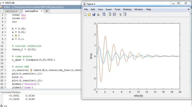
when we run this we will get 2 curves.

1st for displacement which starts at 0 and 2nd is velocity which starts at 3.

clear all
close all
clc

b = 0.05;
g = 9.81;
l = 1
m = 0.1;

% initial condition
theta_0 = [0;3];

% time points
t_span = linspace(0,20,500);

% solve ODE
[t,results] = ode45(@(t,theta)ode_func(t,theta,b,g,l,m),t_span,theta_0)
plot(t,results(:,1))
hold on
plot(t,results(:,2))
xlabel('velocity')
ylabel('time')