Project 2 - Rankine cycle Simulator

Rankine Cycle :

The Rankine cycle is a process widely used by powe plant such as coal fired power plant or nuclear reactors, In this mechanism a fuel is used to produced heat within the boiler converting water into steam which then expands through a turbine producing useful work. This is a thermodynamic cycle which converts into mechanical energy which usually get tranformed electricity by electrical generation.

The step in Rankine cycle as shown in figure and corresponding steps in the pressure volume diagram.

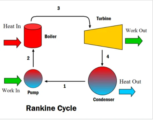
- Pump : Compression to fluid to high pressure using a pump(this takes work)

-Boiler : The compressed fluid is heated to the final temperature which is at boiling point therefore, a phase change occur from liquid to vapour.

- Turbine : Expansion of vapour in turbine

- Condenser : Condensation of the vapor in the condensor where the waste heat goes to the final heat sink(the atmospher or a large body of water)

The efficiency of the Rankine cycle is limited by the high heat of vaporization by the fluid.The fluid must becycled through and reused constanly, therfore, water is the most practicle fluid for the cycle. this is not why many power plants are located near a body of water - that's for the waste heat.

As the water condenses in the condensor waste heat is given of in the form of water vapour which can been seen billowing from a plant's cooling towers. This waste heat is necessary in any thermodynamic cycle. Due to this condensation step, the pressure at the turbine outlet is lowered. This means the pum requires less work to compress the water resulting in higher overall efficiencies.

- Processes of Rankine cycle

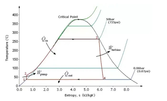
There are 4 processes in the Rankine cycle. The states are identified by numbers in the below T-S diagram

- Process 1 - 2. The working fluid is pumped from low to high pressure.As the fluid is a liquid at the stage the pump requires little energy.

- Process 2-3 The high pressure liquid enters a boiler where it is heated at constant pressure by an external heat source to become a dry saturated vapor. The input energy required can be easily calculated graphically, using enthaly -entropy char, or numerically using steam table.

- process 3 -4 The dry staurated vapor expands through a turbine, generating power. This decreases the temperature and pressure of the vapor and some condensation may occur.The output in this process can easily be calculated using the chart.

- Process 4- 1 The wet vapour then enters a condensor where it is considered at a constant pressure to become a saturated liquid.

Procedure :

1 we will use standard XSteam library to the get the steam table data for water, is given below. It must be used to calculate the points in between the state variables.

2 Cleaning workspace command windows & closing all plots.

3 The user inputs that have to be entered are

Pressure at the turbine inlet(in Bar)

Temperature at the turbine inlet (in Degree C)

Pressure at the condensor (in Bar)

4 Based on the input we will calculate the state variables by using equation and X_steam library whic is a steam table and we can directly read value of state variables using it.

5 After calculating the state variable at each state point we have calculated the turbine and pump work done.

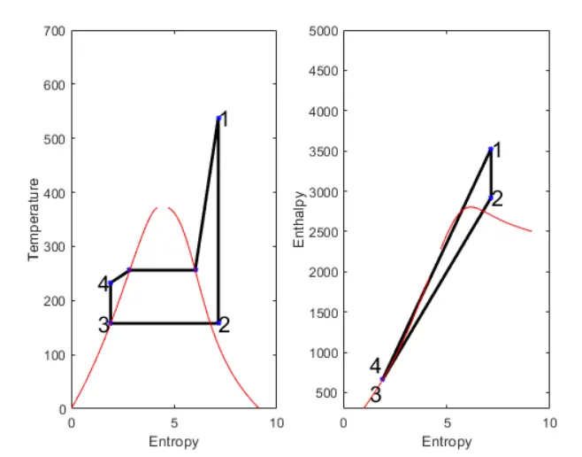
6 At the end we plotted a corresponding T-S and H-S diagram for the given st of inputs.

- Code:

clear all
close all 
clc

% Rankine cycle

fprintf('1-2 Isentropic expansion in turbine')
fprintf('2-3 Constant pressure heat rejection')
fprintf('3-4 Isentropic compression in pump')
fprintf('2-3 Constant pressure heat addition')

% Inputs
p1 = input('enter the pressure at turbine inlet(in bar)');
t1 = input('enter the temperature at inlet(in degree celcius)');
p2 = input('enter the pressure at condenser(in bar)');

fprintf('Result');

% Calculation of Cp value at p1 & p2 for saturated liquid & vapour
Cp1_L=XSteam('CpL_p',p1);
Cp1_V=XSteam('CpV_p',p1);
Cp2_L=XSteam('CpL_p',p2);
Cp2_L=XSteam('CpV_p',p2);

% Calculation of Saturation Temperature at p1 & p2

Tsat_p1=XSteam('Tsat_p',p1)
Tsat_p2=XSteam('Tsat_p',p2)

% Calculation of Enthalpy and Entropy at saturation points

% State point1

Hg_1=XSteam('hV_p',p1);
Sg_1=XSteam('sV_p',p1);

% State point2

Hg_2=XSteam('hV_p',p2);
Sg_2=XSteam('sV_p',p2);

% State point3

Hf_3=XSteam('hL_p',p2);
Sf_3=XSteam('sL_p',p2);

% State point4

Hf_4=XSteam('hL_p',p1);
Sf_4=XSteam('sL_p',p1);

% Calculation of properties at state 1
fprintf('At state point 1n');
fprintf('p1 is :%fbarn',p1);
fprintf('t1 is :%f degCn',t1);

H1=XSteam('h_pT',p1,t1);
fprintf('H1 is :%fkj/kgnn',H1)

S1= XSteam('s_pT',P1,T1);
fprintf('S1 is %f kj/kgnn',S1);

% Calculation of properties at state 2

fprintf('At state point 2n');
fprintf('p2 is %f barn',p2);

S2=S1;
fprintf('S2 is : %fkj/kgkn',S2);

% Calculating the value of x
if (S2<Sg_2)
    x2 = (S2-Sf_3)/(Sg_2-Sf_3);
else
    x2=1;
end
fprintf('x2 is :%n',x2);

% calulating the value of T2

if (x2<1)
    T2 = Tsat_P2;
else
    %S2=Sg_2+Cp2_V*(log(T2/Tsat_p2))
    T2=(Tsat_P2+273.15)*exp(S2-Sg_2)/(Cp2_V);
    T2=T2-273.15;
end

fprintf('T2 is :%f degC n',T2)
if (x2<1)
    H2 = Hf_3+x2*(Hf_3-Hg_2);
else
    H2 = XSteam('h_pT',P2,T2)
end
fprintf('H2is:%f kj/kgnn',H2)

% Calculation of properties at state 2

fprintf('At state point 3n')

P3=P2;
fprintf('P3 is :%fbarn',P3)
V3 = XSteam('vL_p',P3)

T3 = Tsat_P2; 
fprintf('T3 is :%fdegCn',T3)

H3 =Hf_3;
fprintf('H3 is :%f kj/kgnn',H3)

S = Sf_3;
frpintf('S3 is :%f kj/kgnn',S3)

% Calculation of properties at state 2

fprintf('At state point 4n')

P4 = P1
fprintf('P4 is :%f barn',P4)
S4 = S3;
fprintf('S4 is :%f kj/kgnn',S4)

Wp = V3 * (P4 - P3)*100;
H4 = Wp +H3;
fprintf('H4 is :%f kj/kgnn',H4)

T4 = (Tsat_P1 + 273.15)/(exp((Sf_4-S4)/CP1_L));
T4 =T4 -273.15;
fprintf('T4 is :%f Deg celcius nm',T4)

% Calculating and Plotting saturation liquid and vapour lines

temp = linspace(1,T1,1000);
for i = 1:length(temp)
H_L(i) = XSteam('hL_T',temp(i));
H_V(i) = XSteam('hV_T',temp(i));
S_L(i) = XSteam('sL_T',temp(i));
S_V(i) = XSteam('sV_T',temp(i));
end

% Plotting T S Diagram.


figure(1)
hold on

plot([S1,S2],[T1,T2],'g','linewidth',2)
text(S1,T1,'1')
text(S1,T1,'2')

plot([S2 Sg_2],[T2 Tsat_P2],'r','linewidth',2)
text(Sg_2,Tsat_P2,'2s')

plot([S3 Sg_2],[T3 Tsat_P2],'r','linewidth',2)
text(S3,T3,'3')

plot ([S3 S4],[T3 T4],'r','linewidth',2)
text(S4,T4,'4')

plot([S4 Sf_4],[T4 Tsat_P1],'r','linewidth',2)
text(Sf_4,Tsat_P1,'4s')

plot([Sf_4 Sg_1],[Tsat_P1 Tsat_P1],'r','linewidth',2)
text(Sg_1,Tsat_P1,'4s')

plot([Sg_1S1],[Tsat_P1 T1],'r','linewidth',2)
plot(S_L,temp,'b','linestyle','--','linewidth',1)
plot(S_V,temp,'b','linestyle','--','linewidth',1)

title(' T-S Diagram of Ideal Rankine Cycle')
ylabel('Temperature (degC)')
xlable('Specific Entropy(kJ/kgk)')

% Plotting H-S Diagram

figure(2)
hold on
plot([S1 S2],[H1 H2],'r','linewidth',2)
text(S1,H1,'1')
text(S2,H2,'2')

plot([S2 Sg_2],[H2 Hg_2],'r','linewidth',2)
text(Sg_2,Hg_2,'2')

plot([Sg_2 S3],[Hg_2,H3],'r','linewidth',2)
text(S3,H3,'3')

plot([S3 S4],[H3 H4],'r','linewidth',2)
text(S4,H4,'4')

plot([S4,Sf_4],[H4 Hf_4],'r','linewidth',2)
text(Sf_4,Hf_4,'4s')

plot([Sf_4 Sg_1],[Hf_4 Hg_1],'r','linewidth',2)
text(Sg_1,Hg_1,'1s')

plot([Sg_1 S1],[Hg_1 H1],'r','linewidth',2)
plot(S_L,H_L,'b','linestyle','--','linewidth',1)
plot(S_V,H_V,'b','linestyle','--','linewidth',1)
titile('H-S Diagram of Ideal Rankine Cycle')
ylabel('Specific Enthalpy (kJ/Kg)')
xlable('Specific Entropy (kJ/kgK)')

%calculation of work done,heat,SSC and efficiency
wt = H1 -H2;
fprintf('work by turbine is :%f kJ/kgn',Wt)
fprintf('work by compressor is :%f kJ/kgn',Wp)
Wnet = Wt-Wp;
fprintf('Net work done is :%f kJ/kgn',Wnet)
Qin = H1-H4;
eff_thermal =Wnet*100/Qin; 
% Efficiency
fprintf('Thermal efficiency is :%f ',eff_thermal);disp('%')
SSC = 3600/Wt; 
% Specific heat consumption
fprintf('S.S.C is : %f kg/kWh',SSC)