Solving second order ODEs

AIM:

To write a program that solves the Second order ODE.

To write a program in Python that will simulate the pendulum motion.

THEORY:

A simple pendulum is one which can be considered to be a point mass suspended from a string or rod of negligible mass.

In Engineering, ODE is used to describe the transient behavior of a system. A simple example is a pendulum.The way the pendulum moves depends on the Newtons second law. When this law is written down, we get a second order Ordinary Differential Equation that describes the position of the "ball" w.r.t time.

Mathematical Equation

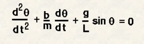
In the above equation,

g = gravity in m/s2,

L = length of the pendulum in m,

m = mass of the ball in kg,

b=damping coefficient

Program Code:

#Solving Second order ODE By Abhishek MB
#Simulation Motion of a Simple Pendulum
import numpy as np
import matplotlib.pyplot as plt
import math
from scipy.integrate import odeint

#functions that returns dz/dt
def model(theta,t,b,g,l,m):

	theta1 = theta[0]
	theta2 = theta[1]
	dtheta1_dt = theta2
	dtheta2_dt = -(b/m)*theta2 - (g/l)*math.sin(theta1)
	dtheta_dt = [dtheta1_dt,dtheta2_dt]
	return dtheta_dt

#Input
b = 0.05  #damping coefficient
g = 9.81  #gravity in m/s^2 
l = 1     #Length of pendulum in m
m = 1   #mass of the ball in kg

#initial conditions
theta_0 = [0,3]

#time points
t = np.linspace(0,20,150)

#solve ODE
theta = odeint(model,theta_0,t,args = (b,g,l,m))

#plot results
plt.plot(t,theta[:,0],'b-',label=r'$\frac{d\theta_1}{dt}=\theta_2 $')
plt.plot(t,theta[:,1],'r--',label=r'$\frac{d\theta_2}{dt}=-\frac{b}{m}\theta_2-\frac{g}{L}sin\theta_1 $')
plt.ylabel('Plot')
plt.xlabel('time')
plt.legend()
plt.show()

#Animation of Simple Pendulum

ct = 1

x0 = 0
y0 = 0

for i in theta[:,0]:
	x1 = (l*math.sin(i))
	y1 = (-l*math.cos(i))

	filename = 'test%05d.png'% ct
	ct = ct + 1

	plt.figure()
	plt.plot([-1,1],[0,0],"black",linewidth=10)
	plt.plot([x0,x1],[y0,y1],"red")
	plt.plot(x1,y1,'o',markersize = 20)
	plt.xlim([-1.5,1.5])
	plt.ylim([-1.5,1.0])
	plt.savefig(filename)
	

Procedure:

>In the start of the program we have to import math and matplotlib for using mathematical operations and graph plotting respectively.numpy was imported for linespace command and for solving differential equation odeint command is used.

>The inputs given in the program is

damping coefficient(b) = 0.05

Length of the pendulum(l) = 1m

mass of the pendulum(m) = 1kg

>The initial displacement and velocity was given 0 and 3 rad/sec respectively by theta_0 array.The time input (0 to 20 sec)was given by the variable t and was split into 150 parts using linespace command.

>A function is definrd in program to calculate angular displacement and velocity at different time intervals.The mathematical equation that is given above is split into two single order differential equation.

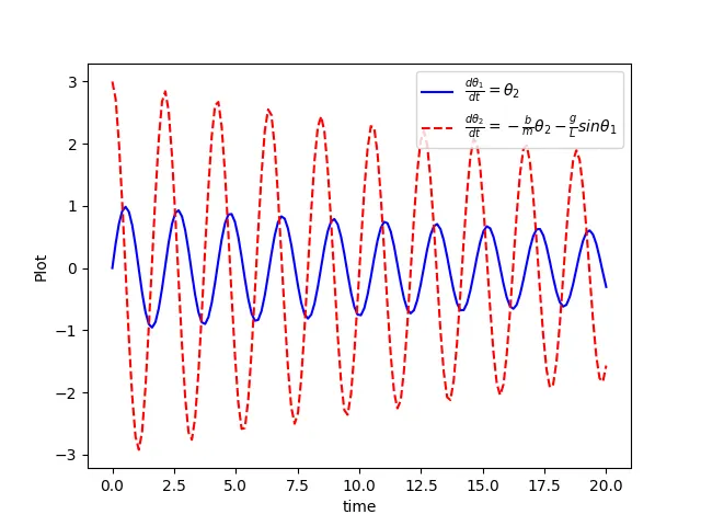
>The displacement and velocity graph against time was plotted using plot command.

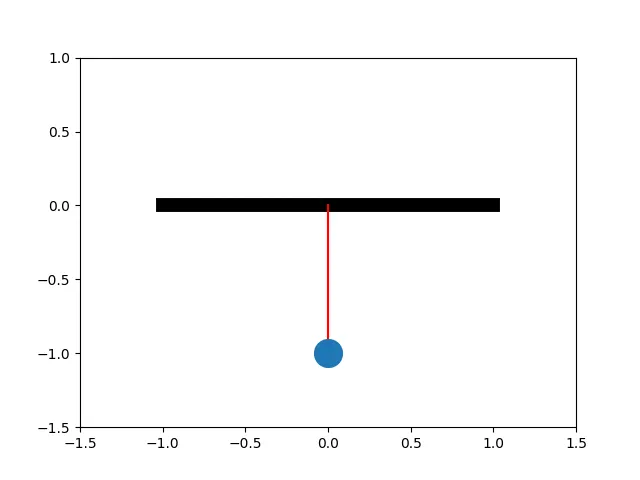
>The multiple images was saved of the motion of the pendulum,these images are stiched in the turned into gif with the help of imagemagick software.

Results:

>The graph shows the variation of angular displacement and velocity with respect to time.

>The amplitude keeps decreasing both in graph and gif as shown below.This is due to damping coefficient given in the inputs.