Week 3 - Solving second order ODEs

Objective: A Matlab program that solves the ODE representing the equation of motion of a simple pendulum with damping

Damped Simple Harmonic motion:

When the motion of an oscillator reduces due to an external force, the oscillator and its motion are damped. These periodic motions of gradually decreasing amplitude are damped simple harmonic motion. An example of a damped simple harmonic motion is a simple pendulum.

In the damped simple harmonic motion, the energy of the oscillator dissipates continuously. But for a small damping, the oscillations remain approximately periodic. The forces which dissipate the energy are generally frictional forces.

This figure shows an idealized pendulum, with a "massless" string or rod of length L and a bob of mass m

ODE representing the equation of motion of a simple pendulum with damping is

here, b represents damping coefficient and g represents acceleration due to gravity

For simulation using Matlab program, we consider the following values

L=1 metre

m=1 kg

b=0.05

g=9.81 m/s2

at time t=0, angular displacement=0 & angular velocity=3 rad/sec

Simulation is for about 0-20sec (we take 500 intervals using linspace command)

Matlab Program code:

Main code

clear all
close all
clc

%Program for solving a second order ODE

%Inputs

%Damping coefficient
b=0.05;
%Acceleration due to gravity in m/s^2
g=9.81;
%Length of string in meters
l=1;
%Mass of pendulum bob in kg
m=1;

%Initial condition
theta0=[0;3];

%Time
time_span=linspace(0,20,500);

%Solve ODE
[t results]=ode45(@(t,theta) odefun(t,theta,b,g,l,m),time_span,theta0);

%Plotting
figure(1)
plot(t,results(:,1))
hold on
plot(t,results(:,2))
xlabel('time')
ylabel('plot')
title('MOTION OF SIMPLE PENDULUM')
legend('Angular displacement','Angular velocity')
hold off

ct=1;
for i=1:length(results(:,1))
    x0=0;
    y0=0;
    x1=l*sin(results(i,1));
    y1=-l*cos(results(i,1));
    
    %Animation
    figure(2)
    plot([-1 1],[0 0],'linewidth',3)
    hold on
    plot([x0 x1],[y0 y1],'linewidth',2,'color','g')
    hold on
    plot(x1,y1,'o','markersize',20,'markerfacecolor','r')
    grid on
    axis([-1.5 1.5 -1.5 0.5])
    pause(0.005)
    hold off
    %Capturing frames to make an animation
    M(ct)=getframe(gcf);
    ct=ct+1;
end

%creating animation movie
movie(M);
videofile=VideoWriter('Simple_pendulum.avi','Uncompressed AVI');
open(videofile);
writeVideo(videofile,M);
close(videofile);

supporting code

%Sub program for solving ODE
function [dtheta_dt]=odefun(t,theta,b,g,l,m)

theta1=theta(1);
theta2=theta(2);
dtheta1_dt=theta2;
dtheta2_dt=-(b/m)*theta2-(g/l)*sin(theta1);
dtheta_dt=[dtheta1_dt;dtheta2_dt];

end

Output:

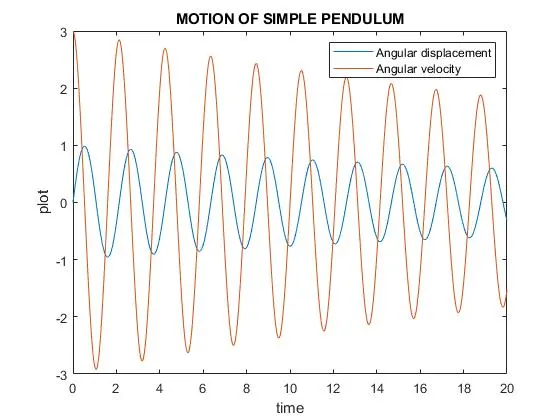
The ode45 solver is an Ordinary Differential Equation solver in MATLAB which is used to solve a differential equation using the Runga-Kutta or R-K method upto 4^th order. This is an inbuilt ODE solver in MATLAB.

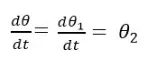
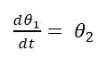
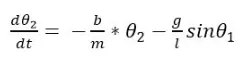
The important thing to remember is that ode45 can only solve a first order ODE. Therefore to solve a higher order ODE, the ODE has to be first converted to a set of first order ODE's.

So, for the above 2nd order ODE, we will make some assumptions like

Let us consider

Then

&

&

Now, the ODE in matrix form will be as

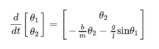
Now matlab code is written to solve this matrix equation in a seperate window and is called in the main program and is solved using ode45 solver.

For simulation, we considered several frames combined together to make an animation/movie.

No major errors were encountered during writing of this program except for some typo errors.