Week 3 - Solving second order ODEs

AIM:

To solve the ODE which represents the equation of motion of a simple pendulum with damping.

OBJECTIVE:

To write a program that solve the following ODE which represents the equation of motion of a simple pendulum with damping and obtain output by solving the ODE.

THEORY:

#The motion of a simple pendulum is the best example for simple harmonic motion

# The pendulum also describes the motion of spring, mass and damper system

#Moment of pendulum is depends on the newtons second law

`(d^2theta) /dt^2 + b/m (d theta)/dt+ g/L sin theta =0`

Where,

g = gravity in m/s^2

l = length of pendulum in metre

m = mass of ball in kg

b = damping co-efficient

The second order differential equation is converted into first order to solve the ODE

where,

`theta = theta1`

`(d theta)/(dt) = (d theta1)/(dt) = theta2`

`(d^2theta)/dt^2 + b/m (d theta)/dt +g/L sin theta = 0`

`(d theta_1)/dt = theta_2 , (d theta_2)/dt=-b/m theta_2 -g/L sin theta_1`

PROGRAM:

To stimulate the transient behaviour of simple pendulum using Matlab

clear all
close all
clc

b = 0.05;
g = 9.81;
l = 1;
m = 1;

%initial condition
theta_0 = [0;3];

%time points
t_span = linspace(0,20,500);

%solve ODE
[t, results] = ode45(@(t,theta)ode_func(t, theta,b,g,l,m),t_span, theta_0);

plot(t,results(:,1))
hold on
plot(t,results(:,2))
ylabel ('Plot')
xlabel ('Time in sec')

%create animation for simple pendulum
fig = 1

for i = 1 :length(t)
    
%initial co-ordiantes
x0 = 0;
y0 = 0;

%final co-ordinates
x1 = 1*sin(results(i,1));
y1 = -1*cos(results(i,1));

%plotting
figure(2)
%base of pendulum
plot ([-1,1],[0,0],'linewidth',5,'color','b')
hold on

%pendulum line
plot([x0,x1],[y0,y1],'linewidth',3,'color','r')
hold on

%pendulum ball
plot(x1,y1,'marker','o','markersize',25,'markerfacecolor','y')
grid on

axis ([-2 2 -2 2]);
pause(0.01);
hold off;
M(fig) = getframe(gcf);
fig  = fig+1;

end

%creating movie from captured frames
 movie(M)
 videofile = VideoWriter('simple_pendulum.avi','uncompressed AVI')
 
 open(videofile);
 writeVideo(videofile,M);
 close(videofile);

FUNCTION PROGRAM:

function[dtheta_dt] = ode_func(t,theta,b,g,l,m)

theta1 = theta(1)
theta2 = theta(2)
dtheta1_dt = theta2;
dtheta2_dt = -(b/m)*theta2 - (g/1)*sin(theta1);
dtheta_dt = [dtheta1_dt; dtheta2_dt];
end

DETAILED EXPLANATION EACH SET OF PROGRAM:

# In first step the input and initial condition are feeded

# In inital condition Angular displacement and Angular velocity are feeded (theta_0 = [0;3])

#Then program is writen the solve the ODE in which MATLAB inbuilt function ode45 is used

[t, results] = ode45(@(t,theta)ode_func(t, theta,b,g,l,m),t_span, theta_0)

#In ode45 constant theta, t, b, g, l, m and other functions are also used

# Solved ODE is plotted using the plot command

# Plot command is used to plot the pendulum line (plot([x0,x1],[y0,y1],'linewidth',3,'color','r') and ball plot(x1,y1,'marker','o','markersize',25,'markerfacecolor','y')

#Then axis and pause commands are given to oscillate the pendulum in its given axis ([-2 2 -2 2])
and in its given pause intervals (0.01)

# Movie command is used to craeate the animated video of damped motion of pendulum.

OUTPUT:

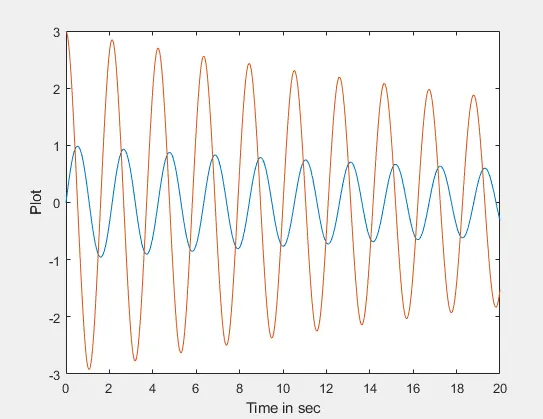
#Angular velocity and Angular velocity plots where generated

#The output obtained is graphical representaion of velocity curve and displacement curve.

#The second video obtained is animated video of damped motion of simple pendulum

Various error are accured during programmimg:

#Spelling mistake in writting function program

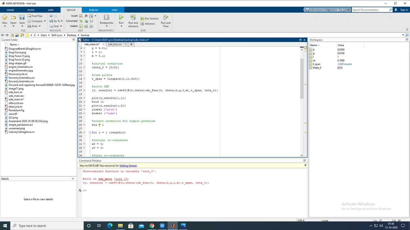
Step taken to overcome this error:

By replacing 'teta_0' to 'theta_0' in [t, results] = ode45(@(t,theta)ode_func(t, theta,b,g,l,m),t_span, theta_0) command.

# Typing mistake in ploting pendulum ball

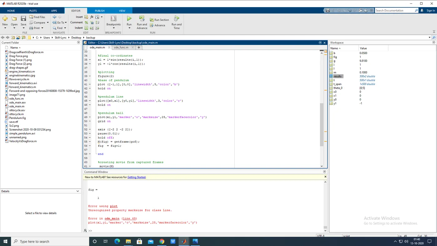
Step taken to overcome this error:

By replacing 'marksize' to 'markersize' in plot(x1,y1,'marker','o','markersize',25,'markerfacecolor','y') command.

CONCLUSION:

Thus the stimulation of the transient behavior of a simple pendulum is succesfully created using MATLAB.