Week 3 - Solving second order ODEs

Solution: Second Order ODEs - Simple Pendulum

Algorithm:

#Second Order ODEs - Simple Pendulum

import numpy as np
import matplotlib.pyplot as plt
import math
from scipy.integrate import odeint

#
# function that returns dz/dt
def model(theta, t, b, g , l, m):
	theta1 = theta[0]
	theta2 = theta[1]
	dtheta1_dt = theta2
	dtheta2_dt = -(b/m)*theta2 - (g/l)*math.sin(theta1)
	dtheta_dt = [dtheta1_dt, dtheta2_dt]
	return dtheta_dt

b = 0.05
g = 9.81
l = 1
m = 1

# initial condition
theta_0 = [0, 3]

# time points
t = np.linspace(0, 10, 150)

# solve ODE
theta = odeint(model, theta_0, t, args = (b, g, l , m))

# plot results
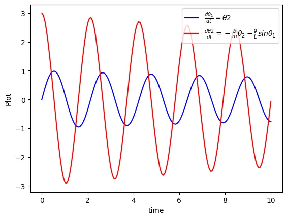
plt.plot(t, theta[:, 0], 'b-', label = r'$\frac{d\theta_1}{dt} = \theta2$', color = 'blue')
plt.plot(t, theta[:, 1], 'b-', label = r'$\frac{d\theta2}{dt} = -\frac{b}{m}\theta_2-\frac{g}{L}sin\theta_1$', color = 'red')
plt.ylabel('Plot')
plt.xlabel('time')
plt.legend(loc = 'best')
plt.show()

print(theta[:, 0])
print(theta[:, 1])

ct = 1

for i in range(0, len(t)):

	x0 = 0
	y0 = 0
	
	# link one link two connector
	x1 = l*math.sin(theta[:, 0][i])
	y1 = -l*math.cos(theta[:, 0][i])

	filename = str(ct) + '.png'
	ct = ct+1

	# to animate plot
	# to plot the plot in a new figure window
	plt.figure()
	plt.plot([x0, x1], [y0, y1])
	plt.plot(x1, y1, 'o', markersize = 10)
	plt.xlim(-1.5, 1.5)
	plt.ylim(-1.5, 1.5)
	# plots one graph and saves figure in the folder same as the code
	plt.savefig(filename)

Output: