Week 3 - Solving second order ODEs

AIM: Write a python program that solve the following ordinary differential equation as function of time. This ODE represents the equation of motion of a simple pendulum with damping.

Objective: The objective of this project is to write a python program that solve the ordinary differential equation of motion of a simple pendulum with damping. Use the output result of this program to make animation of the motion of the pendulum. And upload this animation on YOUTUBE and privide a link in answersheet.

Ordinary Differential Equation (ODE):

An ordinary differential equation, in Mathematics, is an equation which consists of one or more functions of one independent variable along with their derivatives. A differential equation is an equation that contains a function with one or more derivatives. But in the case ODE, the word ordinary is used for derivative of the functions for the single independent variable.

Simple Pendulum

The simple pendulum is an example of a classical oscillating system. Classical harmonic motion and its quantum analogue represent one of the most fundamental physical model. The motion of a simple pendulum is a basic classical example of simple harmonic motion, consisting of a small bob and a massless string.Movement of the pendulum depends on the Newtons second law. When this law is written down,a second order Ordinary Differential Equation is formed that describes the position of the endof the pendulum w.r.t time.

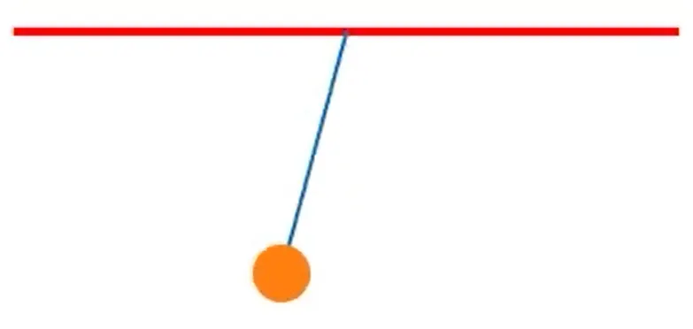
Simple Pendulum

The 2nd order ODE for a simple pendulum with damping is given below.

`(d^2(theta))/dt^2 + (b/m)(d(theta))/dt + (g/l)sintheta = 0 .........eq(1)`

The above equation is 2nd order. To solve this equation(1),first we have to convert this equation into a matrix format so that we can execute in program.

lets assume,

`theta = theta1`

and,

`(d(theta1))/dt = theta2 ........eq(2)`

Therefore equation(1) becomes,

`(d(theta2))/dt + (b/m)*theta2 + (g/l)*sintheta1 = 0`

`(d(theta2))/dt = -(b/m)*theta2 - (g/l)*sintheta1 .........eq(3)`

Where, `theta1 =` angular displacement of the pendulum

`theta2 =` angular velocity of the pendulum

PROCEDURE AND EXPLAINATION:

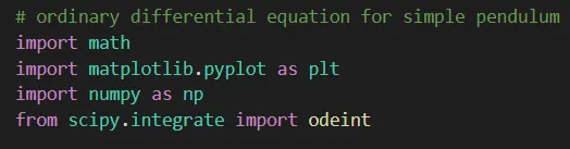
Step-1: Before writing the program first we have to import command to import libraries which will be used in mathematical operation and plotting.

\

Function of the libraries is:

• math library for trignometric equation
• matplotlib library for plotting graphs
• numpy library to use linspace() command which returns evenly spaced samples
• odeint is imported from scipy.integrate library to solve differential equation

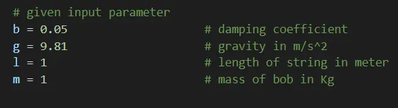
Step-2: Define Input parameter such as mass of the bob, length of string, damping coefficient and gravity.

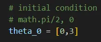
Step-2: Define initial condition and time span

At t = 0, angular displacement for the pendulum is 0 and angular velocity is 3 rad per second.These conditions are stored in an array.

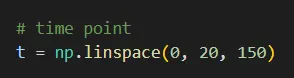
Time span

A time array of 20 sec with 150 intervals is created upon which the ODE will be solved. It is created using numpy module.

Step-3: Define simple pendulum differential function

A function is created which represents the system of differential equation i.e., equation 2 and 3.

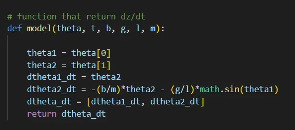
The inputs of this function are theta (empty array which stores solved answers), t (time array), b (damping coefficient), g (gravitational acceleration), l (length of string) and m (mass of bob). `theta1` is the angular displacement and `theta2` is the angular velocity. This function returns an array which has 2 columns and numerous rows. The 1st column is angular displacement and the second column is angular velocity.

Step-4: Solving the ODE's

Using 'odeint' command the ODEs are solved. The 'odeint' is a function in the scipy module which integrates the differential equation upto a time step and after getting that solution it keeps on integrating it. The 'odeint' function is generic means it will choose the best solver based upon the provided system. For 'odeint' command to work properly we pass the differential system function, initial conditions, time span and the arguments.

Step-5: Animation Creation

The 'theta' array contains the solved angular displacement and velocity. Using the 1st column the position of the pendulum is plotted and it is joined to a fixed point to look like a swinging pendulum.The position of the swinging end of the pendulum is calculated using geometry.

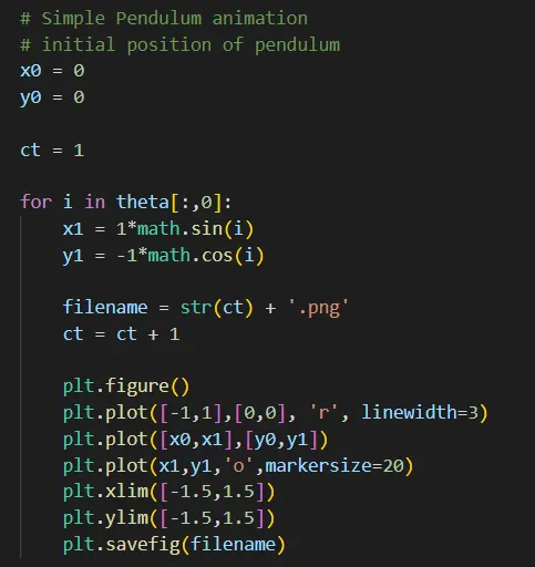
Each figure is saved using 'plt.savefig' command separately with name coresponding to the 'i' value in '.png' format. For creating animation of the pendulum saved plots are stiched together to form animation using external software.

Step-6: Creating Plot

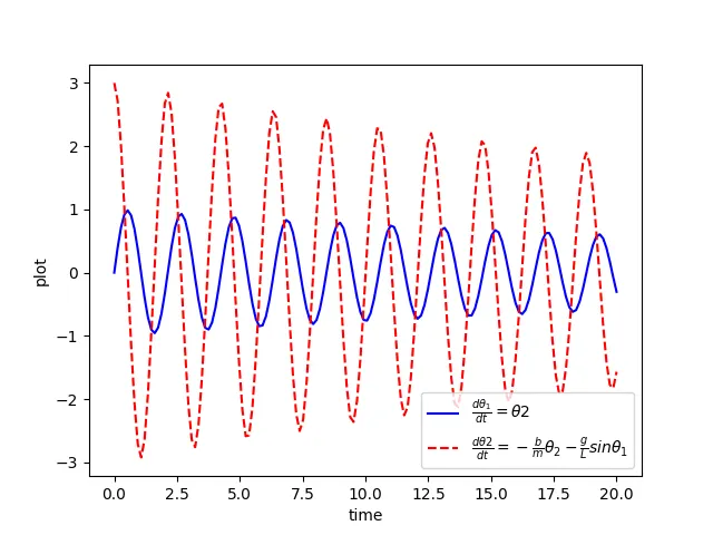
After defining all the terms we need the output so to do that we are using the plot command and plot the graph. Ploting time vs angular displacement graph and time vs angular velocity graph using the 1st and 2nd column of theta array.

After properly arranging the program we get out the desired program.

PYTHON PROGRAM:

CODE

# ordinary differential equation for simple pendulum

importmath

import matplotlib.pyplot as plt

importnumpyasnp

from scipy.integrate import odeint

# function that return dz/dt

def model(theta, t, b, g, l, m):

theta1 = theta[0]

theta2 = theta[1]

dtheta1_dt = theta2

dtheta2_dt = -(b/m)*theta2 - (g/l)*math.sin(theta1)

dtheta_dt = [dtheta1_dt, dtheta2_dt]

return dtheta_dt

# given input parameter

b = 0.05 # damping coefficient

g = 9.81 # gravity in m/s^2

l = 1 # length of string in meter

m = 1 # mass of bob in Kg

# initial condition

# math.pi/2, 0

theta_0 = [0,3]

# time point

t = np.linspace(0, 20, 150)

# solve ODE formula

theta = odeint(model, theta_0, t, args = (b,g,l,m))

# Simple Pendulum animation

# initial position of pendulum

x0 = 0

y0 = 0

ct = 1

for i in theta[:,0]:

x1 = 1*math.sin(i)

y1 = -1*math.cos(i)

filename = str(ct) + '.png'

ct = ct + 1

plt.figure()

plt.plot([-1,1],[0,0], 'r', linewidth=3)

plt.plot([x0,x1],[y0,y1])

plt.plot(x1,y1,'o',markersize=20)

plt.xlim([-1.5,1.5])

plt.ylim([-1.5,1.5])

plt.savefig(filename)

#plot result

plt.plot(t,theta[:,0],'b-',label=r'$\frac{d\theta_1}{dt}=\theta2$')

plt.plot(t,theta[:,1],'r--',label=r'$\frac{d\theta2}{dt}=-\frac{b}{m}\theta_2-\frac{g}{L}sin\theta_1$')

plt.ylabel('plot')

plt.xlabel('time')

plt.legend(loc='best')

plt.show()

OUTPUT RESULT:

Graph between time vs angular displacement and time vs angular velocity

Here, in the above figure we can see that angular velocity (in red color) with respect to time is continuosly decreases due to the damping effect and also the angular displacement graph (in blue color) change its position according to the angular velocity with respect to time.

Simple pendulum result

ffmpeg is used to generate animation file and that file also uploaded in Youtube. to watch this video, follow the link: https://youtu.be/G_pr9bBX_70

Save the plotted file in same folder and open that folder in command window by using copy paste of folder link

Then we use this command in COMMAND PROMPT : "ffmpeg -i %d.png SimplePendulum.avi" or "ffmpeg -i %d.png SimplePendulum.gif" to create animation of png file. Atter pressing enter 'robotic_arm.gif/avi' file name created in that folder.

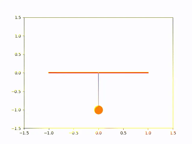
In the case of Python we created the animation by combining the png file of different movement of the bob at different positions.

CONCLUSION

Here, We create a Program for the 2nd order differential equation for simple pendulum, with the help of Python. And also create animation of that whole png file into a gif file and this file upload on youtube, given link: https://youtu.be/G_pr9bBX_70