Week 3 - Solving second order ODEs

AIM

To solves the ODE which represents the equation of motion of a simple pendulum with damping.

OBJECTIVE

Your objective is to write a program that solves the following ODE. This ODE represents the equation of motion of a simple pendulum with damping

THEORY

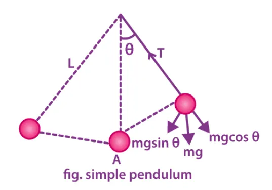
A point mass M is suspended from the end of a light inextensible string whose upper end is fixed to a rigid support. The mass is displaced from its mean position.

assumption

• There is negligible friction from the air and the system
• The arm of the pendulum does not bend or compress and is massless
• The pendulum swings in a perfect plane
• Gravity remains constant

Since the given function is in the second-order differential equation we will convert it into first-order to solve the ODE.

Let
θ=θ1

dθ1/dt=θ2

dθ^2/dt^2=dθ2/dt

Time Period of Simple Pendulum Derivation

Using the equation of motion, T – mg cosθ = mv²L

The torque tending to bring the mass to its equilibrium position,

τ = mgL × sinθ = mgsinθ × L = I × α

For small angles of oscillations sin θ ≈ θ,

Therefore, Iα = -mgLθ

α = -(mgLθ)/I

– ω₀² θ = -(mgLθ)/I

ω₀² = (mgL)/I

ω₀ = √(mgL/I)

Using I = ML², [where I denote the moment of inertia of bob]

we get, ω₀ = √(g/L)

Therefore, the time period of a simple pendulum is given by,

T = 2π/ω₀ = 2π × √(L/g)

INPUTS:

L=1 metre,

m=1 kg,

b=0.05.

g=9.81 m/s2.

Simulate the motion between 0-20 sec,

for angular displacement=0,

angular velocity=3 rad/sec at time t=0

CODE:

import numpy as np
import math
import matplotlib.pyplot as plt
from scipy.integrate import odeint

def model(theta,t,b,g,l,m):
	theta1 = theta[0]
	theta2 = theta[1]
	dthtetha1_dt = theta2
	dtheta2_dt = -(b/m)*theta2-(g/l)*math.sin(theta1)
	dtheta_dt = [dthtetha1_dt,dtheta2_dt]
	return dtheta_dt

b = 0.05
g = 9.8
l = 1
m = 1

theta_0 = [0,3]  #displcement, velocity theta2 = dtheta1/dt


t = np.linspace(0,10,150)

theta= odeint(model,theta_0,t,args=(b,g,l,m))

plt.plot(t,theta[:,0],'b-')
plt.plot(t,theta[:,1],'r--')
plt.xlabel('plot')
plt.ylabel('time')
plt.show()


X0 = 0
Y0 = 0
l = 1

ct=1
for i in theta[:,0]:
	X1 = l*math.sin(i)
	Y1 = -l*math.cos(i)
	ct=ct+1
	filename = str(ct) + '.png'
	plt.figure()
	plt.plot([-1,1],[0,0],'b',linewidth =10)
	plt.plot([X0,X1],[Y0,Y1])
	plt.plot(X1,Y1,'o',markersize =15)
	plt.xlim([-1.5,1.5])
	plt.ylim([-1.5,1.0])
	plt.savefig(filename)
	plt.show()

Step explanation

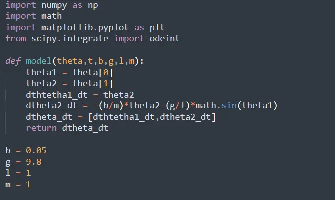
Input the initial conditions of a simple pendulum and define a function for theta matrix with displacement and velocity.

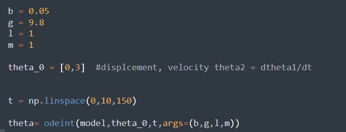
then we define the time-space initial theta and velocity space and call the function.

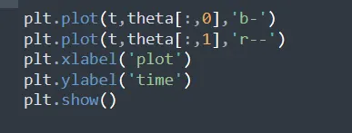
Once we get the theta matrix we plot time vs velocity and displacement.

Once we get these plots, we move ahead with the animation creation. first define the base of the pendulum with X0,Y0 as zero.

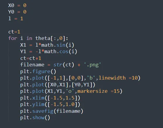
using for loop find values of X1 and Y1 using these coordinates we plot these to make multiple graphs with different theta angles and save them using the filename. now, these images are patched up to make the final animation.

Results.

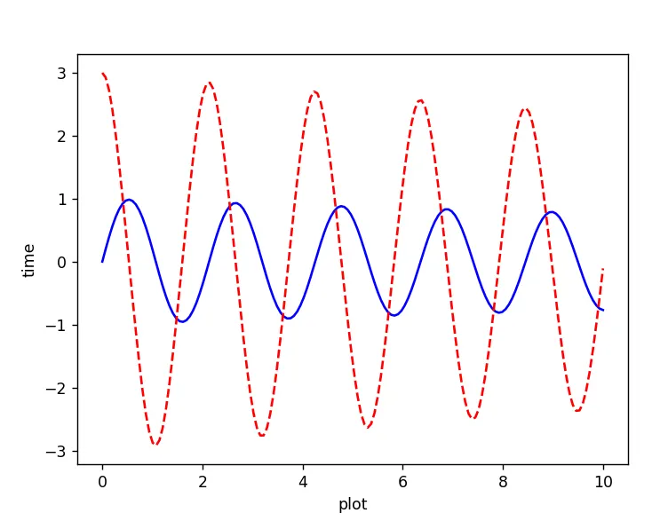
The animation and related graphs are attached given below

Various problems are faced.

1. Spelling mistakes when typing the code.

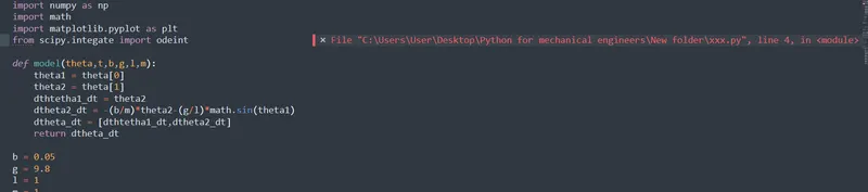
2. mistake in for loop making

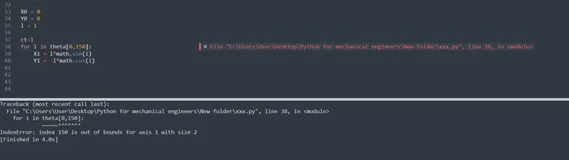
3. the images for animation were not coming.

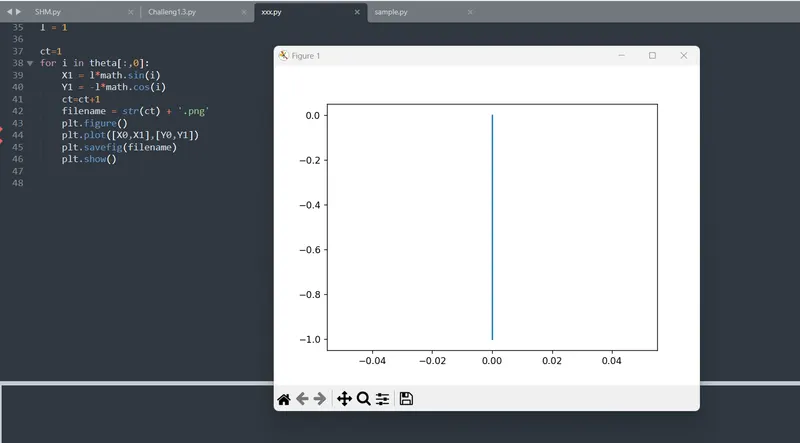
• The step is taken to overcome this error:

1. The spelling mistake was sorted out and given proper spelling

2. The theta was to call from the matrix, not from a definite range say theta[:,0]

3. The error was due to the limits that were not defined so we define x and y limits in the 3rd and 4th quadrants to get the plots.

CONCLUSION.

The code was created for understanding the behavior by plotting a graph and animation.