Week 3 - Solving second order ODEs

AIM: To simulate the transient behavior of a simple pendulum and to create an animation of its motion.

OBJECTIVE :

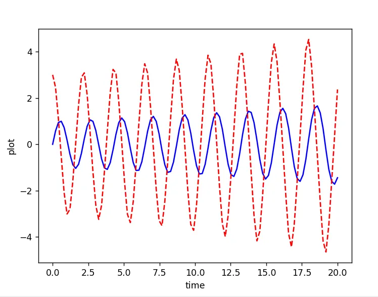
1. To write a program in Python that solves the second-order ODE corresponding to the motion of a simple pendulum and to plot its angular displacement and angular velocity wrt time.

Program-

import math
import matplotlib.pyplot as plt
import numpy
from scipy.integrate import odeint

def model(theta,t,b,g,l,m):
    theta1=theta[0]
    theta2=theta[1]
    dtheta1_dt = theta2
    dtheta2_dt =(b/m)*theta2-(g/l)*math.sin(theta1)
    dtheta_dt = [dtheta1_dt,dtheta2_dt]
    return dtheta_dt
    
b=.05
l=1
m=1
g=9.81
t=numpy.linspace(0,20,100)
p0=[0,3]

theta=odeint(model,p0,t,args=(b,g,l,m))
plt.figure(1)
plt.plot(t,theta[:,0],'b-',label=r'Displacement')
plt.plot(t,theta[:,1],'r--',label=r'Velocity')
plt.xlabel('time')
plt.ylabel('plot')
plt.show()
P = theta[:,0]
ct = 1
x0 = 0
y0 = 0
for i in P:
    x1 = x0+(l*math.sin(i))
    y1 = y0-(l*math.cos(i))
    ct = ct+1
    filename = str(ct) + '.png'
    plt.figure()
    plt.plot([-2, 2], [0, 0], 'b-', linewidth=2)
    plt.plot([x0, x1], [y0, y1])
    plt.plot(x1, y1, marker="o", color='blue', linewidth=2)
    plt.xlim([-1,1])
    plt.ylim([-1,1])
    plt.savefig(filename)

output-

Procedure-

1. importing all imp libraries scipy, matplot , math etc
2. define a function and break the 2nd order ode in two single order ode
3. using the ode int solver pass the values required
4. the first column will have values of all displacement and 2nd will have velocity
5. using plt.plot we can plot the graph
6. to plot the pendulum we know the x0=0 y0=0 and x1 = x0+(l*math.sin(theta)) and y1 = y0-(l*math.cos(i))
7. using a loop till no. of displacement values we can plot pos of pendulum

8. using plot we can plot pos of pendulum and with use of ct variable as string we can save all the plots with diff name

9. now we use ezfig.com to make a gif of all the output images

o/p-

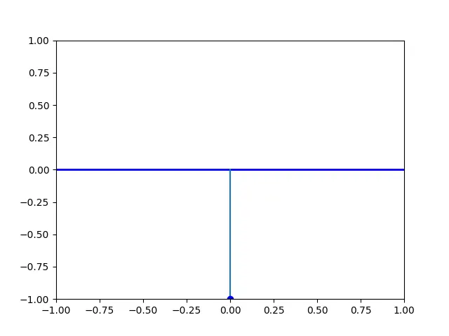
result- pendulum has been plotted