Week 3 - Solving second order ODEs

The governing principle behind the simple movement of a pendulum can be broken down mathematically using a simple Ordinary Differential Equation (ODE). The ODE is given below :

where

θ">θθ = angle between vertical and the string of the pendulum

b= damping coefficient

m= mass of the bob

g= acceleration due to gravity

l= length of the pendulum

python coding for bendulam

import numpy as np
from scipy.integrate import odeint
import matplotlib.pyplot as plt
import math
# input data for bendulam
b=0.05
g=9.8
l=1
m=0.2
# function method for

def model(theta,t,b,g,l,m):
theta1 = theta[0]
theta2 = theta[1]
dtheta1_dt = theta2
dtheta2_dt = -((b/m)*theta2) - ((g/l)*math.sin(theta1));
dtheta_dt=[dtheta1_dt,dtheta2_dt]
return dtheta_dt

# ode solver for 2d order function

theta_0 = [math.pi/2,0]
t=np.linspace(0,20,200)
T=len(t)
theta = odeint(model,theta_0,t,args = (b,g,l,m))

# plt show for given function
plt.figure(1)
plt.plot(t,theta[:,0],'b-',label=r'$\frac{d\theta_1}{dt}=\theta2$')
plt.plot(t,theta[:,-1],'r--',label=r'$\frac{d\theta2}{dt}=-\frac{b}{m}\theta_2-\frac{g}{l}sin\theta_1$')
plt.ylabel('plot')
plt.xlabel('time')
plt.legend(loc='best')
plt.show()
#for loop for degree variation
ct=0
for j in theta[:,0]:
x0=0
y0=0
x1= (l*math.sin(j))
y1= -(l*math.cos(j))
filename = str(ct)+'.png'
ct=ct+1

plt.figure()
plt.plot([x0,x1],[y0,y1],linewidth=3,color='r')
plt.plot(x1,y1,'o',markersize=5)
plt.plot(x1,y1,'o',markersize=15,color='blue')
plt.xlim([-1.5,1.5])#limit X axis
plt.ylim([-1.5,1.5])# limit Y axis
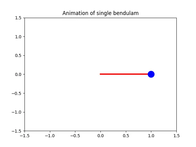
plt.title('Animation of single bendulam')
plt.savefig(filename)

Bendulam plotted images

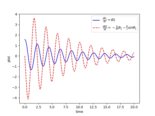
Figure file storing location

Magick animation creation

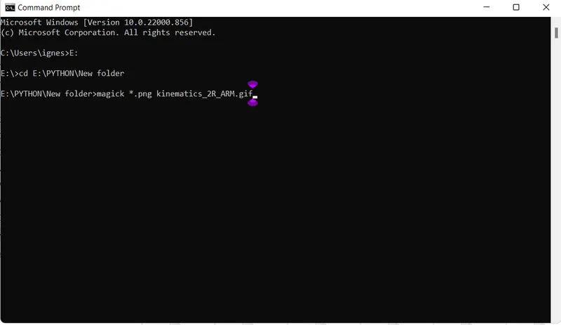
Animation file