Week 3 - Solving second order ODEs

AIM: To simulate the transient behavior of a simple pendulum and to create an animation of its motion.

OBJECTIVE :

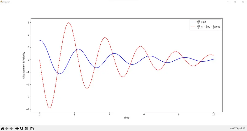
1. To write a program in Python that solves the second order ODE corresponding to the motion of a simple pendulum and to plot its angular displacement and angular velocity wrt time.
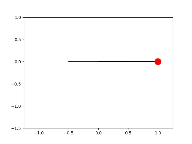
2. To create the animation of the motion of the pendulum by simulating the motion between 0-20 sec, for angular displacement=0, angular velocity=3 rad/sec at time t=0.

THEORY: A simple pendulum is defined to have an object that has a small mass, also known as the pendulum bob, which is suspended from a light wire or string,

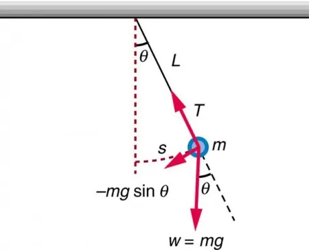
When the bob of the pendulum is displaced from its mean position to either extreme position and is released, the pendulum will swing back and forth with periodic motion until the motion damps. By applying Newton's second law for rotational systems, the equation of motion for the pendulum may be obtained as

τ=I⋅ατ=I⋅α ⇒⇒

−mg⋅sinθ⋅L-mg⋅sinθ⋅L =

mL2⋅d2θdt2mL2⋅d2θdt2

and rearranged as d2θ/dt2+(gL)⋅sinθ=

0d2θdt2+(gL)⋅sinθ=0

and if a damper is introduced in the system the above equations change slightly as

d2θ/dt+(bm)⋅d(θ)dt+(gL)⋅sinθ=

0d2θdt+(bm)⋅d(θ)dt+(gL)⋅sinθ=0

source code:

import math
import matplotlib.pyplot as plt
import numpy as np
from scipy.integrate  import odeint

def model(theta, t, b, l, m, g):
	theta1 = theta[0]
	theta2 = theta[1]
	dtheta1_dt = theta2
	dtheta2_dt = -(b/m)*theta2 - (g/l)*math.sin(theta1)
	dtheta_dt = [dtheta1_dt,dtheta2_dt]
	return dtheta_dt

# Inputs
b = 0.05
l = 1
m = 0.1
g = 9.81

# Initial condition
theta_0 = [(math.pi)/2,0]

# Time points
t = np.linspace(0,10,150)

# Solving the ODE
theta = odeint(model,theta_0,t, args = (b,l,m,g))

# Plotting
plt.figure(1)
plt.plot(t,theta[:,0],'b-',label=r'$\frac{d\theta1}{dt}=\theta2$')
plt.plot(t,theta[:,1],'r--',label=r'$\frac{d\theta2}{dt}=-\frac{b}{m}\theta2-\frac{g}{l}sin\theta1$')
plt.xlabel('Time')
plt.ylabel('Dispacement & Velocity')
plt.legend(loc = 'best')
plt.show()

"""
Animation
"""
x0 = 0
y0 = 0

ct = 1
for i in range(len(t)):
	x1 = x0 + l*math.sin(theta[i,0])
	y1 = y0 - l*math.cos(theta[i,0])

	plt.figure()
	plt.plot([-0.5,0.5],[0,0],'b-')
	plt.plot([x0,x1],[y0,y1],'k-')
	plt.plot(x1,y1,'r',marker='o',markersize='15')
	plt.axis([-1.25,1.25,-1.5,1])
	filename = str(ct) + '.png'
	plt.savefig(filename)
	ct = ct + 1

• First of all, we import the libraries that are going to be used in this program. ‘math’ module for basic math commands, ‘matplotlib.pyplot’ module for plotting purposes, ‘numpy’ module for arrays and ‘odeint’ module from ‘scipy.integrate’ for integrating our second order ODE.
• Before assigning the input values we write a function named ‘model’ with inputs as ‘theta’, ‘time’, ‘b’, ‘g’, ‘l’ and ‘m’. This function breaks our second order ODE into 2 first order ODEs and returns the value of dtheta_dt.
• Then we assign the input values of damping coefficient (b), gravitational acceleration (g), length of pendulum (L) and mass of the bob (m).
• After that we define a variable theta_0 which contains the initial angular displacement = pi/2 and initial angular velocity = 0. After that we assign the value of time span as 0 to 10 sec by the help of linspace command with 150 intervals.
• Now to solve the ODE, we use the command ‘odeint’ which is going to integrate the ODEs and inside the command, we call the function ‘model’ with all the inputs and the arguments.
• Then we use the plot command to generate the plot between displacement and time and velocity and time.
• Now to create an animation of pendulum, first we define the initial values of the coordinates, which is going to be a fixed point. Then we used a ‘for’ loop with loop counter variable (i) with size equal to the length of time (t) array. Also count (ct) variable is also addressed to create separate file for each case.
• Then we define the position of the end point of the string. To create the mass at one end of the pendulum, we use ‘o’ inside the plot command for end point of string, then we choose the color and choose the size by using ‘markersize’ command.
• To name the file in a definite order, we create a variable named ‘filename’ with str of ct and extension as ‘.png’ and use ‘savefig’ command to save the files.
• Now when we run the code, all 150 images are saved in the working folder. We stitched these images together to create the required GIF file.

Result –

1. Displacement and velocity plot with respect to time-

CONCLUSION:

The script writing for 2nd order ode is completed.