Week 3 - Solving second order ODEs
OBJECTIVE:
To write a code in python which solves the second order differential equation for a simple pendulum motion.
PROBLEM STATEMENT:
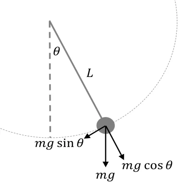
A simple pendulum shows a simple harmonic motion which we need to plot on graph and animate it after writing code in python.
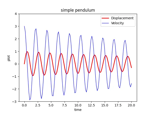
We need to plot a graph showing the velocity and displacement of the bob.
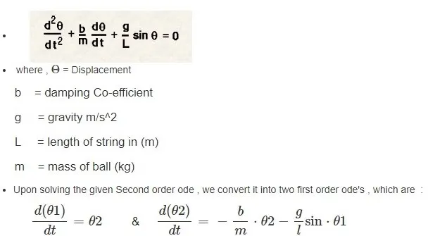
First, we need to know the equation to be used which is shown in the images below.
Second, we need to know the initial conditions to input and the notations.
Lastly, we need to understand how to define the equation and plot the results.
PROCEDURE:
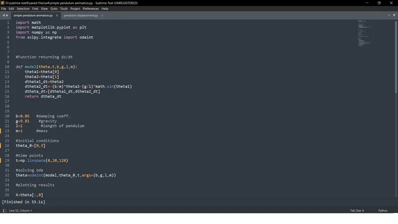
- Input the following libraries-math, matplotlib, numpy and odeint.
- Define returning function dz/dt with converted second order ODE to two first order ODE's as shown in the code and then return the dθ/dt value.
- Enter initial input variables as given in the question as follows-
b=0.05 #damping coeff.
g=9.81 #gravity
l=1 #length of pendulum
m=1 #mass - Take (initial) angular displacement as 0 deg and angular velocity as 3 rad/s.
- Using linspace command define the time interval of 20 seconds and number of iterations as 120.
- Then using the odeint command solve the function defined.
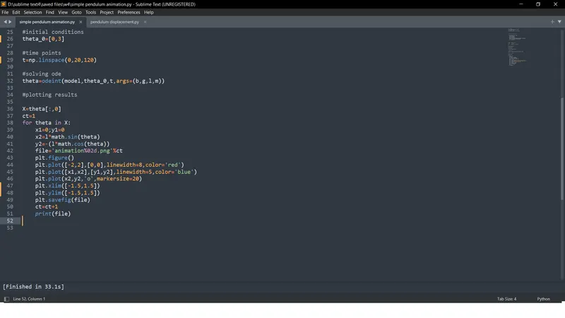
- Finally plot the graph for displacemtent & velocity and for the animation as shown in the code(assume x1=0 & y1=0).
- Also, using cmd prompt create an animation gif for the motion of the pendulum.
PYTHON CODE:
'''
Animation for simple pendulum
By Prithvi
'''

import math
import matplotlib.pyplot as plt
import numpy as np
from scipy.integrate import odeint


#Function returning dz/dt:

def model(theta,t,b,g,l,m):
	theta1=theta[0]
	theta2=theta[1]
	dtheta1_dt=theta2
	dtheta2_dt=-(b/m)*theta2-(g/l)*math.sin(theta1)
	dtheta_dt=[dtheta1_dt,dtheta2_dt]
	return dtheta_dt


#Initial conditions:

b=0.05   #damping coeff.
g=9.81    #gravity
l=1        #length of pendulum
m=1      #mass

theta_0=[0,3]

#Time interval:

t=np.linspace(0,20,120)

#Solving ODE:

theta=odeint(model,theta_0,t,args=(b,g,l,m))

#Plotting results:

X=theta[:,0]
ct=1

for theta in X:
	x1=0;y1=0
	x2=l*math.sin(theta)
	y2=-(l*math.cos(theta))

	file='animation%02d.png'%ct

	plt.figure()

	plt.plot([-2,2],[0,0],linewidth=8,color='red')
	plt.plot([x1,x2],[y1,y2],linewidth=5,color='blue')
	plt.plot(x2,y2,'o',markersize=20)

	plt.xlim([-1.5,1.5])
	plt.ylim([-1.5,1.5])
	plt.savefig(file)

	ct=ct+1
	print(file)
'''
Pendulum Displacement graph
By Prithvi
'''

import math
import matplotlib.pyplot as plt
import numpy as np
from scipy.integrate import odeint


#Function returning dz/dt

def model(theta,t,b,g,l,m):
	theta1=theta[0]
	theta2=theta[1]
	dtheta1_dt=theta2
	dtheta2_dt=-(b/m)*theta2-(g/l)*math.sin(theta1)
	dtheta_dt=[dtheta1_dt,dtheta2_dt]
	return dtheta_dt


#Initial conditions:

b=0.05   #damping coeff.
g=9.81    #gravity
l=1        #length of pendulum
m=1       #mass

theta_0=[0,3]

#Time interval:

t=np.linspace(0,20,120)

#Solving ODE:

theta=odeint(model,theta_0,t,args=(b,g,l,m))

#Plotting results:

plt.plot(t,theta[:,0],label='Displacement',linewidth=2,color='red')
plt.plot(t,theta[:,1],label='Velocity',linewidth=1,color='blue')

plt.ylabel('plot')
plt.xlabel('time')
plt.title('simple pendulum')
plt.xlim(-1,21)
plt.ylim(-3,4)
plt.legend()
plt.show()
OUTPUT:
FOR ANIMATION-
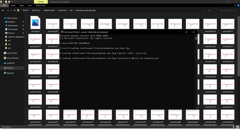
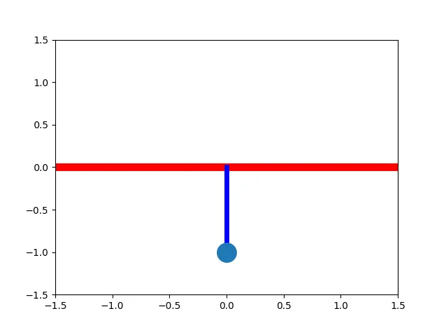
YOUTUBE LINK FOR ANIMATION-
FOR DISPLACEMENT-
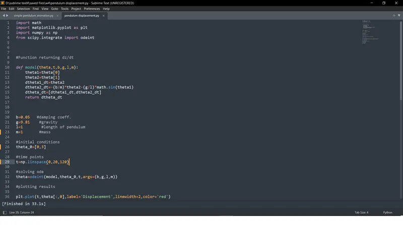
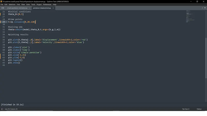
RESULT:
We plotted graphs and created an animation for the ODE defining the simple pendulum motion in python.
DISCUSSIONS:
We used python solver odeint to solve the ODE for a simple pendulum motion.
We noticed that the angular velocity and displacement reduces with time because of damping as visible in the animation and graph.
NOTE: ALL RELATED FILES ARE ATTACHED IN .RAR FORMAT.